Comparison of multiple regression and artificial neural network performances in determining the order of importance of predictors in educational research1,2

Comparación del rendimiento de la regresión múltiple y la red neuronal artificial en la determinación del orden de importancia de los predictores en la investigación educativa

https://doi.org/10.4438/1988-592X-RE-2023-399-568

Emre Toprak  

https://orcid.org/0000-0002-4131-4888 

Erciyes University 

Ömür Kaya Kalkan  

https://orcid.org/0000-0001-7088-4268 

Pamukkale University 

Abstract

Studies aiming to determine the importance rankings of one or more predictor variables on the predicted variable are frequently encountered in education. Multiple Regression (MR) and artificial neural network (ANN) are widely used in this type of research. The present study compares the predictive importance rank performances of MR and ANN methods. For this purpose, two separate real data sets, in which MR assumptions are met and the predictor variables are continuous or discrete, and simulation data generated by considering the relationships in these data sets were used. Absolute relative bias (ARB) and mean square errors (MSE) were used to compare the methods’ performances. The results of the research showed that the increase in sample size had an improving effect on the ARBs and MSEs of the methods. In addition, if the predictors are continuous, researchers may be advised to choose either MR or ANN. However, in cases where the predictors are discrete and the number of predictors is three or more, the use of ANN is recommended. In order to obtain optimal estimations with both methods, it is recommended that researchers use a sample size of at least 200.

Keywords: multiple regression analysis, artificial neural networks, continuous predictor, discrete predictor, order of importance, predictive correlational research.

Resumen

Los estudios que tienen como objetivo determinar los rangos de importancia de una o más variables predictoras en la variable predicha se encuentran con frecuencia en la educación. La regresión múltiple (RM) y la red neuronal artificial (RNA) son ampliamente utilizadas en este tipo de investigación. El presente estudio compara el desempeño del rango de importancia predictiva de los métodos RM y RNA. Para este propósito, dos conjuntos de datos reales separados, en los que se cumplen los supuestos de RM y las variables predictoras son continuas o discretos, y se utilizaron datos de simulación generados al considerar las relaciones en estos conjuntos de datos. Se utilizaron sesgos relativos absolutos (SRA) y errores cuadráticos medios (ECM) para comparar el rendimiento de los métodos. Los resultados de la investigación mostraron que el aumento en el tamaño de la muestra tuvo un efecto de mejora en los SRAs y ECMs de los métodos. Además, si los predictores son continuos, se puede recomendar a los investigadores que elijan RM o RNA. Sin embargo, en los casos en que los predictores sean discretos y el número de predictores sea tres o más, se recomienda el uso de RNA. Para obtener estimaciones óptimas con ambos métodos, se recomienda que los investigadores utilicen un tamaño de muestra de al menos 200.

Palabras clave: análisis de regresión múltiple, redes neuronales artificiales, predictor continuo, predictor discreto, orden de importancia, investigación correlacional predictiva.

Introduction

Predictive type of correlational studies is frequently encountered in the fields of education. In predictive type correlational studies, if there is an adequate correlation between two variables, the score for one variable can be used to predict the score for the other variable (Fraenkel et al., 2011). In these studies, the variable that is estimated can be expressed as the predicted (dependent/criteria) variable, and the variable/s used for the estimation can be expressed as the predictive (independent) variable/s.

In predictive type correlational studies conducted in the fields of education variables related to the cognitive (e.g., Akgül, 2019; Aramburo et al., 2017; Lee, 2016, etc.), affective or psychomotor characteristics (e.g., Arthur & Doverspike, 2001; Atabey, 2020; Ivcevic & Eggers, 2021; Marroquin & Nolen-Hoeksema, 2015, etc.) are addressed. In these studies, the order of importance of the predictor variables on the predicted variable can be determined. In addition, important results revealing the relationships between latent structures (e.g., achievement, motivation, depression, etc.) that cannot be observed directly can be revealed. In this way, a scientific basis can be provided to education researchers, educational practitioners, and decision-makers regarding the issues they need to prioritize and/or improve.

When predictive correlational studies conducted in the fields of education are examined, it is seen that simple and multiple linear regression analyses are mostly used to predict the dependent variable (e.g., Akhtar & Herwig, 2019; Alandete, 2015; Bergold & Steinmayr, 2018; Garcini et al., 2013; Teressa & Bekele, 2021, etc.). However, regression analyses have many assumptions that need to be met, and there may be situations where not all of these assumptions are met. This situation reveals the need to employ different methods in prediction studies. One of the methods that can be used as an alternative to multiple regression (MR) analysis in prediction studies is artificial neural networks (ANNs). ANN has been used in social sciences, engineering, business, and many other fields (e.g., Bayru, 2007; Cansız et al., 2020; Okkan & Mollamahmutoğlu, 2010; Tolon, 2007, etc.) for a long time, it has recently been used frequently in educational research (e.g., Kalkan & Coşguner, 2021; Moreetsi & Mbako, 2008; Toprak & Gelbal, 2020, etc.). The MR and ANN methods used in the research are briefly introduced below.

Multiple regression (MR)

Regression analyses are a set of statistical techniques that allows evaluating the relationship between a dependent variable and one or more independent variables (Tabachnick & Fidell, 2013). MR is concerned with predicting a dependent variable based on a set of estimators (Stevens, 2009). In addition, MR allows for determining the total variance explained by the predictor variables on the dependent variable, examining the statistical significance of the predictor variables, and interpreting the relationship between the predictor variables and the dependent variable (Büyüköztürk, 2014). In addition, MR is a quite efficient technique for analyzing the total and separate effects of predictor variables on a dependent variable (Pedhazur, 1997).

In MR, the predictive variables should be continuous variables at least on an interval scale; however, discrete variables can also be included in the analysis after they are defined as dummy variables (Büyüköztürk, 2014). In addition, MR has some assumptions to be met, such as normality, linearity, homoscedasticity of residuals, independence of errors, multicollinearity, adequate sample size, and examination of outliers (Tabachnick & Fidell, 2013).

Artificial neural networks (ANNs)

The beginning of ANN studies, which is based on the working principle of the human brain, dates back to the 1940s. ANNs are also expressed as computer programs that imitate biological neural networks in the human brain, in the form of simulating the biological nervous system (Elmas, 2003). A biological nerve cell consists of four essential components: dendrite, nucleus, axon, and synapse (Öztemel, 2012). Similarly, an artificial neuron consists of the inputs created by the information coming from the outside world, the weights by which the importance level of the information is determined, the sum function that provides the calculation of the net information entering the cell, and the activation function that determines the output to be produced (Baş, 2006; Öztemel, 2012).

Some advantages are effective in the widespread use of ANN. These can be listed as being able to solve complex problems, adapting to new situations with minor changes, generalizing based on the results obtained, being faster than traditional statistical methods, working with incomplete data, handling defective or multidimensional data with error tolerance, and pattern recognition in missing data (Çırak & Çokluk, 2013; Haykin, 1994; Öztemel, 2012; Simpson, 1990). These advantages of ANN make it preferable to regression-based methods.

There are studies in the literature conducted for the purpose of comparing the prediction performances of MR and ANN. In these studies, the performances of the methods were examined over different parameters such as mean squares of error, percentages of prediction, coefficients of determination, and scatter diagrams (e.g., Akbilgiç & Keskintürk, 2008; Cansız et al., 2020; Gorr et al., 1994; Lykourentzou et al., 2009; Okkan & Mollamahmutoğlu, 2010; Turhan et al., 2013; Zaidah & Daliela, 2007, etc.). To the best of our knowledge, no research has been found that examines the performance of both methods in determining the order of importance of predictor variables on real and simulation datasets based on predictor type, the number of predictors, and sample size. Therefore, the results of the research can contribute to the determination of the limitations of the methods in practice; in addition, it is thought that it can provide inferences for researchers and practitioners. For that reason, the present study aims to compare the priority rankings obtained from MR and ANN, in determining the order of importance of the variables over real and simulation datasets of different sample sizes consisting of continuous or discrete variables. For this purpose, answers to the following research questions (RQ) were sought:

RQ1. What are the relationships between variables in real datasets consisting of continuous or discrete predictive variables?

RQ2. When predictor variables are continuous;

a. What is the order of importance obtained by MR and ANN from the real dataset?

b. How does the order of importance, absolute relative bias (ARB), and mean square error (MSE) obtained by MR and ANN from simulation datasets with different sample sizes (100, 200, 400, 800) and the number of predictors (2, 3, 4) change?

RQ3. When predictor variables are discrete;

a. What is the order of importance obtained by MR and ANN from the real dataset?

b. How does the order of importance, ARB, and MSE obtained by MR and ANN from simulation datasets with different sample sizes (100, 200, 400, 800) and the number of predictors (2, 3, 4) change?

Method

Study group

Within the scope of the research, two different real datasets belonging to the studies of Toprak and Kalkan (2019a, 2019b) were used to compare the performance of the MR and ANN methods in determining the order of importance of the continuous and discrete variables. The first dataset consists of the answers given by 445 students (324 female, 121 male) enrolled at three different high schools in Turkey (Toprak & Kalkan, 2019a). This dataset was used to compare the order of importance of the methods when the predictor variables were continuous.

The second dataset consists of the answers given by 992 students (540 female, 452 male) enrolled in five different secondary schools in Turkey (Toprak & Kalkan, 2019b). This dataset was used to compare the ordering of the methods when the predictor variables were discrete.

Data collection instruments

The first dataset of the present study consists of the Cognitive Flexibility Scale, Coping Strategies Scale, and Competency Expectation Scale scores used by Toprak and Kalkan (2019a) in their research. These scales are introduced below, respectively.

Cognitive flexibility scale

The scale developed by Martin and Rubin (1995) and adapted into Turkish by Çelikkaleli (2014) consists of 12 items. The Cronbach Alpha (Cr α) reliability coefficient of the scale was .71. The scale has a one-dimensional factor structure.

Coping strategies scale

The scale, developed by Spirito et al. (1988) and adapted into Turkish by Bedel et al. (2014), consists of 11 items and three sub-dimensions: active coping, avoidant coping, and negative coping. The Cr α reliability coefficient of the scale was .72 for active coping, .70 for avoidant coping, and .65 for negative coping.

Competency expectation scale

The scale, which was developed by Muris (2001) and adapted into Turkish by Çelikkaleli et al. (2006), consists of 23 items and three sub-dimensions: academic competence expectation, social competence expectation, and emotional competence expectation. The Cr α reliability coefficient was reported as .64 for academic competence expectation, .69 for emotional competence expectation, and .71 for social competence expectation.

The second dataset of the present research consists of the data obtained by Toprak and Kalkan (2019b) with the personal information form in their studies. This information form and the variables included in the study are briefly introduced below.

Personal information form

This form consists of discrete variables determined as predictors of mathematics course achievement scores, such as gender, family income level, mother’s education level, and father’s education level (Table I).

TABLE I. Descriptive statistics on the predictors of mathematics course achievement scores

Variables		f	%
Gender	Female	540	54.4
	Male	452	45.6
Family income level	2000 Turkish Lira (TL) and below	220	22.2
	2001-4000 TL	414	41.7
	4001-6000 TL	197	19.9
	6001 TL and above	161	16.2
Mother’s education level	Up to primary school	280	28.2
	Secondary school	259	26.1
	High school	279	28.1
	Undergraduate and above	174	17.5
Father’s education level	Up to primary school	166	16.7
	Secondary school	247	24.9
	High school	290	29.2
	Undergraduate and above	289	29.1

Data analysis

MR and ANN methods were used to determine the order of importance of the variables. For this purpose, two different real datasets and simulation datasets generated by considering these datasets were used. Missing data, adequacy of sample size, and outlier analysis were performed to evaluate the fitting of real data sets for MR, and normality, linearity, homoscedasticity of residuals, independence of errors, multicollinearity assumptions were tested.

Mahalanobis distances obtained in determining the outliers were compared with the chi-square critical value (α = .001). While evaluating the adequacy of the sample size, the number of predictors x 15 proposed by Stevens (2009) and 50 + 8 x the number of predictors proposed by Tabachnick and Fidell (2013) were taken into account. Normal probability plots (P-P) and scatter plots of regression standardized residuals were used to control the assumptions of normality, linearity, and covariance of residuals. In determining the multicollinearity problem, bivariate correlation, tolerance, condition index (CI), and variance inflation factor (VIF) values were considered. Real data and simulation data were used in MR and ANN analyses.

Real data

Two different datasets were used for real data analysis. In dataset1, all variables are continuous, and the dependent variable is cognitive flexibility. Social competence expectations, academic competence expectations, emotional competence expectations, and active coping variables were used to predict cognitive flexibility (Toprak & Kalkan, 2019a).

In dataset2, the dependent variable is the mathematics course achievement scores (continuous variable). Discrete variables of gender, family income, father’s education level, and mother’s education level were used as predictors of mathematics course achievement scores (Toprak & Kalkan, 2019b).

Simulation design

R software (Core team, 2017) was used to generate simulation data. 24 (2 x 4 x 3) study conditions were created by crossing 2 variable types (continuous, discrete), 4 sample sizes (100, 200, 400, 800), and 3 number of predictors (2, 3, 4) and one hundred datasets were generated for each study condition.

Using the variance, covariance, and mean values obtained from the real dataset (dataset1) consisting of continuous variables, simulation data were generated. SimDesign (Chalmers & Adkins, 2020) package was used to generate these datasets.

Using the correlation, mean, and standard deviation values obtained from the real dataset (dataset2) consisting of discrete predictors, simulation data were generated. The OrdNor (Amatya & Demirtas, 2015) package was used to generate these data. The values of the dependent variable (mathematics course achievement scores) in the generated datasets were rounded to the nearest integer and limited to the range of 0-100 to be fitted with the real values.

Discrete predictors were coded as dummy variables and included in the analysis. The first category for each variable was determined as the reference group (Table I). In determining the order of importance of the discrete variables, the mean of the standardized coefficients obtained from all categories of the relevant variable except the reference group was taken into account.

In order to compare the performance of the methods, the order of importance of the variables, ARB, and MSE were used. Parameter values obtained from real datasets were assumed as true values, and ARB was calculated with estimations obtained from simulation data. The following formula was used to calculate ARB (Bandalos & Leite, 2013).

The mean square error (MSE) formula was used to determine the efficiency of parameter estimations (Bandalos & Leite, 2013).

In Equations 1 and 2, is jth sample estimation of the ith true parameter value is the replication number. ARB can be interpreted as percent ARB by multiplying it by 100.

The R was used for the MR analysis, and the statistical program for social sciences (SPSS; IBM, 2020) was used for the ANN analysis. Multilayer Perceptron Model was used in ANN analysis; 70% of the datasets were chosen as training samples and 30% as the test sample. The hyperbolic tangent function was used for the cells in the hidden layer, and the softmax function was used for the cells in the output layer. Different training and test data are used in each analysis made with ANN. For this reason, each dataset in the relevant condition was analyzed 100 times to ensure stability.

Results

The adequacy of sample size, outliers, normality, linearity, homoscedasticity of residuals, and multicollinearity (e.g., tolerance, condition index, variance inflation factor, etc.) assumptions were examined before performing MR analyses, and it was seen that these assumptions were met. Then, the results related to the research problems are presented respectively.

Correlation between variables in real datasets consisting of continuous or discrete predictor variables

The bivariate correlations between the variables in the real datasets are presented in Table II, respectively.

TABLE II. Correlations in the real dataset consisting of continuous and discrete variables

Continuous Variables	CF	ESC	EAC	EEC	AC
CF	–
ESC	.439**	–
EAC	.424**	.306**	–
EEC	.425**	.418**	.338**	–
AC	.401**	.291**	.379**	. 483**	–
Discrete Variables	MCAS	G	FI	FEL	MEL
MCAS	–
G	-.201**	–
FI	.307**	.016	–
FEL	.320**	-.067**	.425*	–
MEL	.324**	-.031**	.457**	.589**	–

**p<.01; *p<.05. Note. CF: cognitive flexibility; ESC: expectation of social competence; EAC: expectation of academic competence; EEC: expectation of emotional competence; AC: active coping; MCAS: mathematics course achievement scores; G: gender; FI: family income; FEL: father’s education level; MEL: mother’s education level.

Table II shows that there is a positive, moderate level, and significant correlation between CF and ESC, EAC, EEC, and AC. The variable with the highest correlation with CF was ESC; the variable with the lowest correlation is AC. In addition to this, there is a positive, moderate level, and significant correlation between MCAS and FI, FEL, and MEL, and a negative, low level and significant correlation with G. The variable with the highest correlation with MCAS is MEL; the variable with the lowest correlation is G.

Results for continuous predictors

The order of importance and standardized coefficients obtained with MR and ANN in conditions where there are 2, 3, and 4 continuous predictors in the real dataset (dataset1) are presented in Table III.

TABLE III. MR and ANN’s order of importance in the real dataset consisting of continuous predictors

DV	Method	NP	Predictors’ order of importance and standardized coefficients (in brackets)
CF	MR	2	1.	ESC (0.34)	2.	EAC (0.32)
		3	1.	EAC (0.27)	2.	ESC (0.26)	3.	EEC (0.22)
		4	1.	ESC (0.25)	2.	EAC (0.23)	3.	EEC (0.16)	4.	AC (0.16)
	ANN	2	1.	ESC (0.50)	2.	EAC (0.49)
		3	1.	EAC (0.35)	2.	ESC (0.34)	3.	EEC (0.31)
		4	1.	ESC (0.30)	2.	EAC (0.29)	3.	EEC (0.21)	4.	AC (0.20)

Note. DV: dependent variable; NP: number of predictors.

Table III shows that for the conditions with two and four predictors in predicting CF, ESC is the variable with the highest importance level according to both methods. In the prediction with three variables, although the importance order of the predictor variables is the same in terms of methods, the variable with the highest importance level is EAC. These results show that both methods reveal the same order for the condition where the predictor variables are continuous, regardless of the number of predictors. The order of importance and standardized coefficients obtained by MR from simulation datasets with the different number of predictors and sample sizes are presented in Table IV.

TABLE IV. MR’s order of importance and standardized coefficients in simulation datasets consisting of continuous predictor

DV	NP	SS	Predictors’ order of importance and standardized coefficients (in brackets)
CF	2	100	1.	ESC (0.34)	2.	EAC (0.32)
		200	1.	ESC (0.34)	2.	EAC (0.31)
		400	1.	ESC (0.34)	2.	EAC (0.32)
		800	1.	ESC (0.34)	2.	EAC (0.32)
	3	100	1.	EAC (0.27)	2.	ESC (0.26)	3.	EEC (0.23)
		200	1.	ESC (0.27)	2.	EAC (0.26)	3.	EEC (0.22)
		400	1.	EAC (0.27)	2.	ESC (0.25)	3.	EEC (0.23)
		800	1.	EAC (0.27)	2.	ESC (0.26)	3.	EEC (0.23)
	4	100	1.	ESC (0.24)	2.	EAC (0.23)	3.	EEC (0.18)	4.	AC (0.17)
		200	1.	ESC (0.26)	2.	EAC (0.22)	3.	EEC (0.17)	4.	AC (0.16)
		400	1.	ESC (0.25)	2.	EAC (0.23)	3.	EEC (0.17)	4.	AC (0.16)
		800	1.	ESC (0.25)	2.	EAC (0.23)	3.	EEC (0.17)	4.	AC (0.16)

Note. SS: sample size.

Table IV shows that the variable with the highest significance level according to the MR results obtained from two predictors in different sample sizes is ESC. In the condition that the number of predictors is four, the variable with the highest importance level is again ESC. In addition, in conditions with two and four predictors, the order of importance of the predictors is the same for all sample sizes. On the other hand, in the conditions with three predictors, ESC is the variable with the highest importance level for the sample size of 200; it is EAC for sample sizes of 100, 400, and 800. In addition, for this condition, EEC is the least important variable in all sample sizes. The order of importance obtained for all predictors is generally fitted with the real data (Table III). The order of importance and standardized coefficients obtained by ANN from simulation datasets with different number of predictors and sample sizes are presented in Table V.

TABLE V. ANN’s order of importance and standardized coefficients in simulation datasets consisting of continuous predictors

DV	NP	SS	Predictors’ order of importance and standardized coefficients (in brackets)
CF	2	100	1.	ESC (0.52)	2.	EAC (0.48)
		200	1.	ESC (0.52)	2.	EAC (0.48)
		400	1.	ESC (0.52)	2.	EAC (0.48)
		800	1.	ESC (0.51)	2.	EAC (0.49)
	3	100	1.	ESC (0.35)	2.	EAC (0.34)	3.	EEC (0.31)
		200	1.	ESC (0.35)	2.	EAC (0.34)	3.	EEC (0.31)
		400	1.	EAC (0.35)	2.	ESC (0.34)	3.	EEC (0.31)
		800	1.	EAC (0.35)	2.	ESC (0.34)	3.	EEC (0.31)
	4	100	1.	ESC (0.27)	2.	EAC (0.26)	3.	EEC (0.24)	4.	AC (0.22)
		200	1.	ESC (0.30)	2.	EAC (0.26)	3.	EEC (0.23)	4.	AC (0.21)
		400	1.	ESC (0.29)	2.	EAC (0.27)	3.	EEC (0.22)	4.	AC (0.21)
		800	1.	ESC (0.30)	2.	EAC (0.28)	3.	EEC (0.21)	4.	AC (0.20)

Table V shows that ESC is the variable with the highest importance level according to the ANN results obtained from two and four predictors in different sample sizes. In addition, in conditions with two and four predictors, the order of importance of the predictors is the same for all sample sizes. On the other hand, in the condition with three predictors, ESC is the variable with the highest importance level for sample sizes of 100 and 200; it is EAC for sample sizes of 400 and 800. In addition, for this condition, EEC is the least important variable in all sample sizes. The order of importance obtained for all predictors is generally fitted with the real data (Table III).

The ARBs of the parameter estimations obtained by MR and ANN from simulation datasets with different numbers of continuous predictors and sample sizes are presented in Figure I.

FIGURE I. ARBs obtained by MR and ANN in simulation datasets consisting of continuous predictors

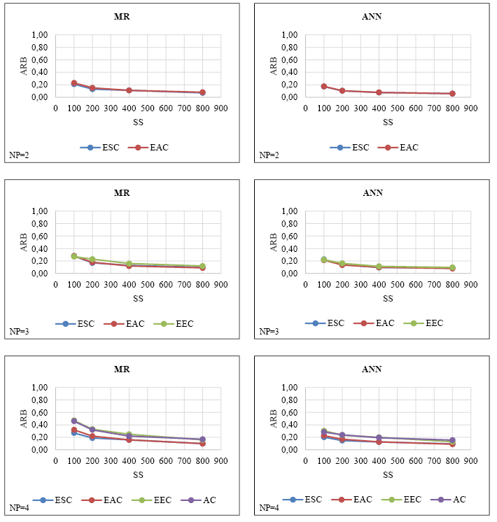
Figure I shows that ARB decreases as the sample size increases for both methods, regardless of the number of predictors. While dramatic decreases were observed in ARB, specifically in the transition from 100 to 200 sample sizes, these decreases were lower in larger samples (i.e., 400-800). In addition, for all predictors, the highest ARBs were observed at a sample size of 100 and the lowest ARBs at a sample size of 800. When MR and ANN ARB means were compared, it was determined that ANN had lower ARB averages, regardless of the number of predictors. However, since the ARB averages of both methods are over 10% for all numbers of predictors (Flora & Curran, 2004), it can be said that these estimates have substantial bias.

On the other hand, the increase in the number of predictors while the sample size was fixed, caused an increase in the ARB means of both methods. However, the increase in ANN ARB means was lower in comparison to MR. It should be noted that these increases in the ARB means were more dramatic, specifically in small sample sizes.

The MSEs of the parameter estimations obtained by MR and ANN from simulation datasets with different numbers of continuous predictors and sample sizes are presented in Figure II.

FIGURE II. MSEs obtained by MR and ANN in simulation datasets consisting of continuous predictors

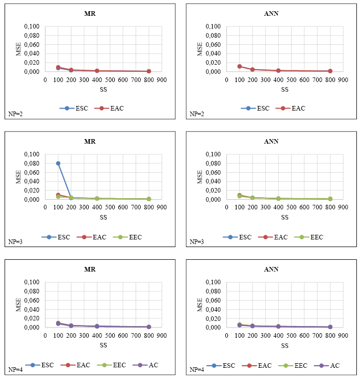
Figure II shows that for both methods, regardless of the number of predictors, MSE decreases as the sample size increases. Generally, dramatic decreases were observed in MSE in transitions from 100 to 200 sample sizes; in larger samples (i.e., 400-800), these decreases were lower. In addition, for all predictors, the highest MSE values were observed at a sample size of 100, and the lowest MSEs at a sample size of 800. When MR and ANN MSEs were compared, it was determined that ANN had lower MSEs, except when the number of predictors was two.

On the other hand, as the number of predictors increased, no important change was observed in the MSEs of the methods (except NP=3, ESC). In addition, it can be said that MSEs have quite similar values in samples of 200 and above.

Results for discrete predictors

The order of importance and standardized coefficients obtained with MR and ANN in conditions where there are 2, 3, and 4 discrete predictors in the real dataset are presented in Table VI.

TABLE VI. MR and ANN’s order of importance in the real dataset consisting of discrete predictors

DV	Method	NP	Predictors’ order of importance and standardized coefficients (in brackets)
MCAS	MR	2	1.	FI (0.25)	2.	G (0.21)
		3	1.	G (0.19)	2.	FI (0.17)	3.	FEL (0.13)
		4	1.	G (0.19)	2.	FI (0.14)	3.	FEL (0.09)	4.	MEL (0.09)
	ANN	2	1.	FI (0.27)	2.	G (0.20)
		3	1.	G (0.16)	2.	FI (0.15)	3.	FEL (0.13)
		4	1.	G (0.14)	2.	FI (0.10)	3.	MEL (0.09)	4.	FEL (0.08)

Table VI shows that for the condition with two predictors in predicting MCAS, the predictor with the highest importance level according to both methods was FI and that G for conditions with three and four predictors. In addition, for the conditions where the number of predictors is 2 and 3, the order of importance obtained by both methods is the same; it was seen that only the third and fourth-order changed when the number of predictors was 4. The order of importance and standardized coefficients obtained by MR from simulation datasets with the different number of predictors and sample sizes are presented in Table VII.

TABLE VII. MR’s order of importance and standardized coefficients in simulation datasets consisting of discrete predictors

DV	NP	SS	Predictors’ order of importance and standardized coefficients (in brackets)
MCAS	2	100	1.	FI (0.28)	2.	G (0.18)
		200	1.	FI (0.28)	2.	G (0.21)
		400	1.	FI (0.26)	2.	G (0.20)
		800	1.	FI (0.27)	2.	G (0.19)
	3	100	1.	FI (0.21)	2.	FEL (0.20)	3.	G (0.17)
		200	1.	FI (0.20)	2.	G (0.19)	3.	FEL (0.19)
		400	1.	G (0.19)	2.	FEL (0.18)	3.	FI (0.18)
		800	1.	FEL (0.19)	2.	FI (0.19)	3.	G (0.18)
	4	100	1.	FI (0.18)	2.	FEL (0.17)	3.	G (0.17)	4.	MEL (0.15)
		200	1.	G (0.19)	2.	FI (0.17)	3.	FEL (0.14)	4.	MEL (0.12)
		400	1.	G (0.19)	2.	FI (0.15)	3.	FEL (0.13)	4.	MEL (0.12)
		800	1.	G (0.18)	2.	FI (0.15)	3.	FEL (0.13)	4.	MEL (0.12)

Table VII shows that FI is the predictor with the highest importance according to the MR results obtained from two predictors at different sample sizes. When the number of predictors was three, the predictor with the highest importance level differentiated according to the sample sizes. In the case where the number of predictors is four, the predictor with the highest importance level in sample sizes of 200 and above is G. While the importance rankings obtained from the conditions with two and four predictors were generally congruent with the real data importance rankings (Table VI); no such agreement was observed in conditions where the number of predictors was three. The order of importance and standardized coefficients obtained by ANN from simulation datasets with the different number of predictors and sample sizes are presented in Table VIII.

TABLE VIII. ANN’s order of importance and standardized coefficients in simulation datasets consisting of discrete predictors

DV	NP	SS	Predictors’ order of importance and standardized coefficients (in brackets)
MCAS	2	100	1.	FI (0.26)	2.	G (0.21)
		200	1.	FI (0.26)	2.	G (0.22)
		400	1.	FI (0.26)	2.	G (0.21)
		800	1.	FI (0.27)	2.	G (0.19)
	3	100	1.	FI (0.16)	2.	G (0.14)	3.	FEL (0.14)
		200	1.	G (0.16)	2.	FI (0.15)	3.	FEL (0.14)
		400	1.	G (0.15)	2.	FI (0.15)	3.	FEL (0.14)
		800	1.	FI (0.16)	2.	FEL (0.14)	3.	G (0.13)
	4	100	1.	G (0.11)	2.	FI (0.10)	3.	MEL (0.09)	4.	FEL (0.09)
		200	1.	G (0.13)	2.	FI (0.10)	3.	FEL (0.09)	4.	MEL (0.09)
		400	1.	G (0.13)	2.	FI (0.10)	3.	MEL (0.09)	4.	FEL (0.09)
		800	1.	G (0.12)	2.	FI (0.10)	3.	MEL (0.09)	4.	FEL (0.09)

Table VIII shows that FI is the predictor with the highest importance level according to the ANN results obtained from different sample sizes with two predictors. When the number of predictors was three, the predictor with the highest importance level differentiated according to the sample sizes. For the condition where the number of predictors was four, the predictor with the highest importance level is G. When all conditions are taken into account (except NP=3, SS=100 and 800; NP=4, SS=200), the predictive importance rankings obtained from the simulation datasets were generally congruent with the real data importance rankings (Table VI).

The ARBs of the parameter estimations obtained by MR and ANN from simulation datasets with different numbers of discrete predictors and sample sizes are presented in Figure III.

FIGURE III. ARBs obtained by MR and ANN in simulation datasets consisting of discrete predictors

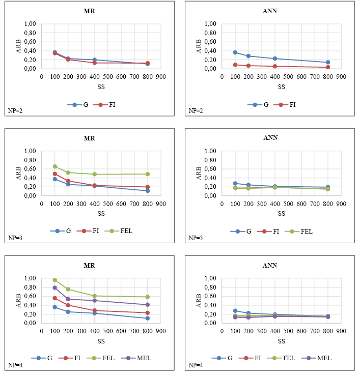
Figure III shows that the ARB generally decreases as the sample size increases for both methods, regardless of the number of predictors. In addition, ANN ARBs were less affected by the increase in sample size in comparison to MR. Generally, dramatic decreases were observed in ARB, specifically in the transition from 100 to 200 sample sizes, these decreases were lower in larger samples (i.e., 400-800). In addition, for all predictors in MR, the highest ARBs were observed with a sample size of 100 and the lowest ARBs

with a sample size of 800. On the other hand, a common pattern related to the increase in sample sizes was not detected in the ANN ARBs. For example, while the increase in sample size remediates the gender predictor’s ARBs, it did not have the same effect on the ARBs of other variables (FI, FEL, MEL). When the MR and ANN ARB means were compared, it was determined that ANN had lower ARBs, regardless of the number of predictors. Since the ARB averages of both methods are over 10% for all predictor numbers (Flora & Curran, 2004), it can be said that these estimations have substantial bias.

On the other hand, when the sample size is fixed, the increase in the number of predictors led to an increase in the MR ARB means; no such common pattern (i.e., increase, decrease) was observed for ANN ARB means. In addition, it is noteworthy that the deterioration in ARB means is more dramatic, specifically in small sample sizes.

The MSEs of the parameter estimations obtained by MR and ANN from simulation datasets with different numbers of discrete predictors and sample sizes are presented in Figure IV.

FIGURE IV. MSEs obtained by MR and ANN in simulation datasets consisting of discrete predictors

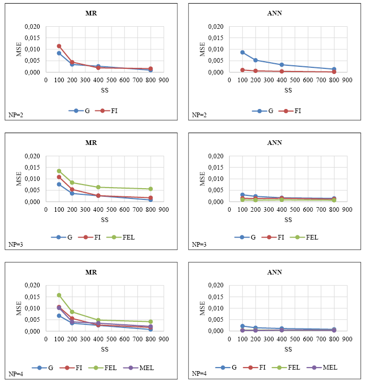
Figure IV shows that the MSE generally decreases as the sample size increases for both methods, regardless of the number of predictors. In addition, ANN MSEs were less affected by the increase in sample size in comparison to MR. Generally, dramatic decreases were observed in MSEs of the MR, specifically in the transition from 100 to 200 sample sizes, these decreases were lower in larger samples (i.e., 400-800). On the other hand, MSEs of ANN were not generally affected by the increase in sample size. In addition, it can be said that for all predictors in both methods, the highest MSEs were observed in a sample size of 100, and the lowest MSEs were observed in a sample size of 800. When MR and ANN MSEs were compared, it was determined that ANN generally had lower MSEs, regardless of the number of predictors.

In general, ANN MSEs decreased while MR MSEs increased as the number of predictors increased. In addition, it is noteworthy that the deterioration in MR MSEs is more dramatic, specifically in small sample sizes.

Discussion

In this study, MR and ANN performances were compared in determining the order of importance of the predictor variables. For this purpose, real datasets and simulation data were used. The type of variable, sample size, and the number of predictors were manipulated in the simulation study. First, the correlations between the variables in the real datasets and the MR assumptions were examined. Then, the methods’ performances were compared over their predictors’ order of importance, ARB, and MSE.

Comparison of predictors importance rankings of methods

When the predictors’ importance rankings obtained from the real dataset in which the predictors are continuous are compared, it is seen that the rankings of both methods are the same regardless of the number of predictors. The importance rankings obtained from the simulation datasets are the same as the real data importance rankings, except for one simulation condition for MR and two for ANN.

On the other hand, when the predictors’ importance rankings obtained from the real dataset in which the predictors are discrete are compared, the importance rankings obtained by both methods are the same for the conditions where the number of predictors is two and three. In the condition that the number of predictors is four, only the third and fourth ranks have changed. Since this change is caused by a value less than 0.01, it can be stated that it is not very important. Therefore, it can be said that the methods have almost the same rankings. The importance rankings obtained from the simulation datasets are the same as the real data importance rankings, except for five simulation conditions for MR and three for ANN. In addition, it should be noted that MR may not perform real data importance rankings when the number of predictors is three.

In summary, in the present study, it can be said that the methods perform the same order of importance if the predictors are continuous and that they perform quite similar order of importance if the predictors are discrete. Turhan et al. (2013) performed MR and ANN to the dataset consisting of continuous and discrete predictors and reported that the same variable was the best predictor according to both methods. It can be stated that this finding supports the findings of the present research.

Comparison of ARBs of methods

In conditions where the predictors are both continuous and discrete, as the sample size increases, the ARB of the methods decreases regardless of the number of predictors. This remediate effect of the increase in sample size is specifically greater when transitioning from 100 to 200. In addition, when the ARB means are compared, it can be said that ANN outperforms MR, regardless of the number of predictors. On the other hand, it should be noted that the methods perform predictions with substantial bias (>10%; Flora & Curran, 2004).

On the other hand, in conditions where the predictors are continuous, while the sample size is fixed, the increase in the number of predictors leads to an increase in the ARB means of the methods. In general, the increase in MR ARB means is higher in comparison to ANN. In the conditions where the predictors are discrete, while the sample size is fixed, the mean of the MR ARB increases as the number of predictors increases. However, no such common pattern (i.e., increase, decrease) is determined in ANN. In addition, the increases in the mean of ARB are higher, specifically in small sample sizes, in conditions where the predictors are both continuous and discrete. Considering the ARB means, it can be stated that ANN outperforms MR.

Comparison of MSEs of methods

In conditions where the predictors are both continuous and discrete, the MSEs of the methods tend to decrease as the sample size increases, regardless of the number of predictors. This remediate effect of the increase in sample size reaches its maximum level, specifically when the sample size is increased from 100 to 200. In addition to this, it is quite low in other sample transitions. When the mean MSEs of the methods are compared, it can be said that ANN generally outperforms MR. Lykourentzou et al. (2009) and Turhan et al. (2013), who compared different variables that predict student achievement in the field of educational sciences, revealed that ANN performs better predictions than MR. Altun et al. (2019) estimated the graduation grades of classroom teaching students using MR and ANN and determined that both methods (MR=94.30%, ANN=94.43%) provided very close results. On the other hand, when the studies comparing the methods in the field of business over MSEs are examined, Akbilgiç and Keskintürk (2008); Aktaş et al. (2003), and Yüzük (2019) reported that ANN outperformed MR. When the studies comparing the methods in the field of engineering over MSEs are examined, Okkan and Mollamahmutoğlu (2010) state that ANN outperforms MR whereas Cansız et al. (2020) reported that MR outperformed ANN.

On the other hand, when the number of predictors increases while the sample size is fixed, no important change is determined in the MSEs of the methods in the conditions where the predictors are continuous. The MSEs of the methods are quite similar, specifically in the sample size of 200 or more. In the conditions where the predictors are discrete, when the number of predictors increases while the sample size is fixed, the MR MSEs increase in general; ANN MSEs, on the other hand, tend to decrease. It should be noted that increases in MR MSEs are more dramatic, specifically in small sample sizes.

Conclusion and Suggestions

Generally, the increase in sample size, regardless of the predictor type (i.e., continuous and discrete) and the number of predictors, remediates the ARBs and MSEs of the methods. In order to obtain optimal estimations with both methods, it is recommended to use a sample size of at least 200. However, it should be noted that the estimates obtained for this sample size may have moderate bias.

In case the predictors are continuous, researchers may prefer one of the two methods since the predictor order of importance of the methods is the same. However, in cases where the predictors are discrete and the number of predictors increases (specifically>2), ANN can be recommended due to its superior performance.

On the other hand, when the predictors are continuous, the increase in the number of predictors leads to a deterioration of the ARB means of the methods. However, it should be noted that this deterioration is more dramatic in MR. In case the predictors are discrete, ANN provides more robust estimations than MR.

While the predictors are continuous, the increase in the number of predictors does not lead to an important change in the MSEs of the methods. The MSEs of the methods are quite similar, specifically in sample sizes of 200 or more. When the estimators are discrete, the increase in the number of estimators generally leads to a deterioration in the MSEs of the MR, while the MSEs of the ANN are affected slightly.

As a result, when ARB and MSEs are considered, ANN outperforms MR. For this reason, it can be suggested that researchers prefer ANN firstly. MR is a reasonable alternative to ANN if the predictors are continuous and their assumptions are met. However, it should be noted that MR may not perform well even if its assumptions are met if the predictors are discrete. Specifically, in the case of three or more discrete predictors, it may be recommended for researchers to use ANN. In addition to this, it should be emphasized that an important advantage of ANN is that it does not need the assumptions required by MR.

It is important for educational research to reveal estimation methods that allow for determining the order of importance of the predictors in different models. Therefore, it can be assumed that studies in which methods are addressed comparatively have the potential to contribute to other studies in the field of education. In this context, the results of the present study provide a better understanding of the functioning of MR and ANN, which contributes to educational research, under different conditions.

The present research has been carried out on two different real datasets where the assumptions of the MR are met and the predictor variables are continuous or discrete. The simulation data was generated by considering the relationships in these datasets. This research design can be considered as a limitation of the present research. In addition, it should be noted that another limitation is that the predictors explain the total variance in the dependent variable in the real sets, which is 34.3% and 20.4%, respectively. To the best of our knowledge, since there are no studies comparing both methods in the field of education under conditions such as variable type, sample size, and the number of predictors, more research is needed to generalize the results. In future studies, data can be generated by modeling relationships in larger samples, and method comparisons can be performed through models in which continuous and discrete predictors combined are used.

References

Akbilgiç, O., & Keskintürk, T. (2008). The comparison of artificial neural networks and regression analysis. Istanbul Management Journal, 19(60), 74-83.

Akgül, S. (2019). Predictive power of mathematical self-efficacy for gifted and talented students’ mathematical achievement. EKEV Journal, 23(78), 481-496.

Akhtar, M., & Herwig, B. K. (2019). Coping styles and socio-demographic variables as predictors of psychological well-being among international students belonging to different cultures. Curr Psychol, 38, 618-626.

Aktaş, R., Doğanay, M., & Yıldız, B. (2003). Financial failure prediction: Statistical methods and artificial neural network comparison. Ankara University SBF Journal, 58, 1-24.

Alandete, J. G. (2015). Does meaning in life predict psychological well-being? An analysis using the Spanish versions of the purpose-in-life test and the Ryff’s scales. The European Journal of Counselling Psychology, 3(2), 89-98.

Amatya, A., & Demirtas, H. (2015). OrdNor: An R package for concurrent generation of correlated ordinal and normal data. Journal of Statistical Software, 68, 1-14.

Altun, M., Kayıkçı, K., & Irmak, S. (2019). Estimation of graduation grades of primary education students by using regression analysis and artificial neural networks. e-IJER, 10(3), 29-43.

Aramburo, V., Boroel, B., & Pineda, G. (2017). Predictive factors associated with academic performance in college students. Social and Behavioral Sciences, 237, 945-949.

Arthur, W., & Doverspike, D. (2001). Predicting motor vehicle crash involvement from a personality measure and a driving knowledge test. Journal of Prevention & Intervention in the Community, 22(1), 35-42.

Atabey, N. (2020). Future expectations and self-efficacy of high school students as a predictor of sense of school belonging. Education and Science, 45(201), 125-141.

Bandalos, D. L., & Leite, W. (2013). The use of Monte Carlo studies in structural equation modeling research. In G. R. Hancock & R. O. Mueller (Eds.), Structural equation modeling: A second course (pp. 385-426). Information Age Publishing.

Baş, N. (2006). Artificial neural networks approach and an application (Unpublished master’s thesis). Mimar Sinan Fine Arts University.

Bayru, P. (2007). Electronic media consumer choice analysis: Artificial neural networks to evaluate the performance of the model with lojit (Unpublished doctoral dissertation). Istanbul University.

Bedel, A., Işık, E., & Hamarta, E. (2014). Psychometric properties of the KIDCOPE in Turkish adolescents. Education and Science, 39(176), 227-235.

Bergold, S., & Steinmayr, R. (2018). Personality and intelligence interact in the prediction of academic achievement. Journal of Intelligence, 6(2), 27.

Büyüköztürk, Ş. (2014). Sosyal bilimler için veri analizi el kitabı [Manual of data analysis for social sciences]. Pegem Yayıncılık.

Cansız, Ö. F., Öztekin, N., & Erginer, İ. (2020). Comparison of artificial neural networks and multi-variable linear regression techniques in determination of the number of optimum vehicles. DUMF Journal, 11(2), 771-782.

Chalmers, R. P., & Adkins, M. C. (2020). Writing effective and reliable Monte Carlo simulations with the SimDesign package. The Quantitative Methods for Psychology, 16(4), 248-280.

Çelikkaleli, Ö. (2014). The validity and reliability of the cognitive flexibility scale. Education and Science, 39(176), 339-346.

Çelikkaleli, Ö., Gündoğdu, M., & Kıran-Esen, B. (2006). Questionnaire for measuring self-efficacy in youths: Validity and reliability study of Turkish form. EJER, 25, 62-72.

Çırak, G., & Çokluk, Ö. (2013). The usage of artifical neural network and logistic regression methods in the classification of student achievement in higher education. MJH, 3(2), 71-79.

Elmas, Ç. (2003). Yapay sinir ağları [Artificial neural networks]. Seçkin Kitabevi.

Flora, D. B., & Curran, P. J. (2004). An empirical evaluation of alternative methods of estimation for confirmatory factor analysis with ordinal data. Psychological Methods, 9(4), 466-491.

Fraenkel, J. R., Wallen, N., & Hyun, H. (2011). How to design and evaluate research in education. McGraw Hill.

Garcini, L. M., Short, M. B., & Norwood, W. D. (2013). Affective and motivational predictors of perceived meaning in life among college students. The Journal of Happiness and Well-Being, 1(2), 47-60.

Gorr, W. L., Nagin, D., & Szczypula, A. (1994). Comparative study of artificial neural network and statistical models for predicting student grade point averages. International Journal of Forecasting, 10(2), 17-34.

Haykin, S. (1994). Neural networks: A comprehensive foundation. Macmillan Press.

IBM. (2020). IBM SPSS statistics base 25. SPSS Inc.

Ivcevic, Z., & Eggers, C. (2021). Emotion regulation ability: Test performance and observer reports in predicting relationship, achievement and well-being outcomes in adolescents. IJERPH, 18(6), 3204.

Kalkan, Ö. K., & Coşguner, T. (2021). Evaluation of the academic achievement of vocational school of higher education students through artificial neural networks. Gazi University Journal of Science, 34(3), 851-862.

Lee, J. (2016). Attitude toward school does not predict academic achievement. Learning and Individual Differences, 52, 1-9.

Lykourentzou, I., Giannoukos, I., Mpardis, G., Nikolopoulos, V., & Loumos, V. (2009). Early and dynamic student achievement prediction in e-learning courses using neural networks. JASIST, 60(2), 372–380.

Marroquin, B., & Nolen-Hoeksema, S. (2015). Event prediction and affective forecasting in depressive cognition: Using emotion as information about the future. Journal of Social and Clinical Psychology, 34(2), 117-134.

Martin, M. M., & Rubin, R. B. (1995). A new measure of cognitive flexibility. Psychological Reports, 76, 623-626.

Moreetsi, T., & Mbako, M. T. (2008). Predicting students’ performance on agricultural science examination from forecast grades. US-China Education Review, 5(10), 45-51.

Muris, P. (2001). A brief questionnaire for measuring self-efficacy in youths. Journal of Psychopathology and Behavioral Assessment, 23(3), 145-149.

Okkan, U., & Mollamahmutoğlu, A. (2010). Daily runoff modeling of Yiğitler stream by using artificial neural networks and regression analysis. Dumlupınar University Journal of Science Institute, 23, 33-48.

Öztemel, E. (2012). Yapay sinir ağları [Artificial neural networks]. Papatya Yayıncılık.

Pedhazur, E. J. (1997). Multiple Regression in behavioral research, explanation and prediction. Thomson Learning.

R Core Team. (2017). R: A language and environment for statistical computing [Computer Software]. R Foundation for Statistical Computing.

Simpson, P. K. (1990). Artificial neural systems foundations, paradigms, application and implementation. Pergamon Press.

Spirito, A., Stark, L. J., & Williams, C. (1988). Development of a brief coping checklist for use with pediatric populations. Journal of Pediatric Psychology, 13, 555-574.

Stevens, N. (2009). Applied multivariate statistics for the social sciences. Taylor and Francis.

Tabachnick, B. G., & Fidell, L. S. (2013). Using multivariate statistics. Pearson.

Teressa, T. D., & Bekele, G. (2021). Motivational predictors of tenth graders’ academic achievement in Harari secondary schools. IJELS, 9(3), 9-19.

Tolon, M. (2007). Measuring customer satisfaction with artificial neural networks and an application of retail consumers in Ankara (Unpublished doctoral dissertation). Gazi University.

Toprak, E., & Gelbal, S. (2020). Comparison of classification performances of mathematics achievement at PISA 2012 with the artificial neural network, decision trees and discriminant analysis. IJATE, 7(4), 773-799.

Toprak, E., & Kalkan, Ö. K. (2019a, June). Ergenlerde bilişsel esnekliğin yordayıcısı olarak başa çıkma stratejileri ve yetkinlik inançları [Coping strategies and self-efficacy beliefs as predictors of cognitive flexibility in adolescents]. 6. EJER Congress, Ankara.

Toprak, E., & Kalkan, Ö. K. (2019b, Haziran). Matematik başarısını yordayan değişkenlerin yapay sinir ağları ile incelenmesi [Examining the variables that predict mathematics achievement with artificial neural networks]. 2. IBAD Congress, İstanbul.

Turhan, K., Buırçin, K., & Engin, Y. Z. (2013). Estimation of student success with artificial neural networks. Education and Science, 38(170), 112-120.

Yüzük, F. (2019). Multiple regression analysis and neural networks with Turkish energy demand forecast (Unpublished master’s thesis). Cumhuriyet University.

Zaidah, I., & Daliela, R. (2007). Predicting students’ academic performance: Comparing artificial neural network, decision tree and linear regression. 21st Annual SAS Malaysia Forum, Kuala Lumpur.

Information address: Emre Toprak. Erciyes University, Faculty of Education, Department of Educational Sciences. Postal code 38039, Kayseri, Turkey. E-mail: etoprak@erciyes.edu.tr 

---