What happened with PISA 2018 in Spain? An explanation based on response times to items

¿Qué pasó en España con PISA 2018? Una explicación a partir de los tiempos de respuesta a los ítems

https://doi.org/10.4438/1988-592X-RE-2025-411-727

José G. Clavel

Universidad de Murcia

https://orcid.org/0000-0001-5800-319X

Francisco Javier García-Crespo

Universidad Complutense de Madrid

https://orcid.org/0000-0002-1050-462Y

Luis Sanz San Miguel

Instituto Nacional de Evaluación Educativa (INEE)

https://orcid.org/0000-0002-1050-462X

Abstract

Keywords:

PISA 2018, Reading fluency, rapid guessing, process data, odd behaviour, loglinear model, Reading performance

Resumen

Palabras clave:

Introduction

On November 19, 2019, the OECD issued an official announcement stating that Spain’s Reading results would not be released together with those of the other countries on December 3, 2019. The announcement said:

“Spain’s data met PISA Technical Standards with no apparent technical errors or manipulations identified. However, the data show implausible student-response behaviour. Consequently, the OECD is unable to assure full international comparability of Spain’s results at this moment. Spain has agreed to follow the OECD’s recommendation to defer the publication of its results and data while possible sources of those anomalies are investigated”.

Months later, on July 23, 2020, Spain’s reading results were published, along with a brief independent study (Annex A9) that offered possible explanations for the detected anomalies. The study pointed out, among other factors, that the timing of when the PISA test was conducted in Spain could have influenced the results. In the same document, it was also noted that the impact of one section of the test, Reading Fluency, might have been more significant than initially expected:

“The analysis of Spain’s data also reveals how the inclusion of reading fluency items may have strengthened the relationship between test performance and student effort in PISA more generally. The OECD is therefore exploring changes to the administration and scoring of reading fluency items to limit the occurrence of disengaged response behaviour and mitigate its consequence”.

Apparently, the anomalous behaviour of some students in the Reading Fluency items (hereinafter RF) triggered the unexpected results in some Autonomous Communities, leading to not publishing Spain´s PISA 2018 reading results in December 2019. But... What characteristics do the students who exhibited this anomalous behaviour have? Why did this problem occur in some Autonomous Communities and not in others? What could have caused this behaviour? We will attempt to answer these questions in the following study using the published PISA 2018 reading results.

Our work falls within the category of those who analyse the data available since the tests are conducted on a tablet, as in the case of PISA 2018 (Goldhammer et al. 2020). Indeed, computer-based assessments have had several methodological consequences. Among other things, it has made it possible to design adaptive tests that change according to students´ responses (as is the case with PISA tests); it has made it possible to design response items that were not technically possible before; and, above all, it has allowed to polish test evaluation by incorporating all the collateral information available into the model (see, for example, Bezirhan et al., 2020). Our work falls within this third area: we use the computer trace (log-files) generated by the student as they progress through the test (process data) and combine it with their answers (response data). For a review of how the two sources of information are being integrated into LSAs such as PISA, see Anghel et al (2024).

According to the test, these log files may include information such as which keys were pressed or how the cursor moved across the screen, and in more advanced assessments, even data on eye movements or heart rate for each item and each participant. In PISA 2018, the log files collected response times: excessively short times would be a sign of rapid guessing behaviour when answering (Wise, 2017). This would reveal the test-taker disengagement (Avvisati et al, 2024), which is a risk in tests such as PISA, where students have nothing at stake (what the literature refers to as a low-stakes context).

A second source of information available in PISA 2018 is non-response to certain items. As pointed out by Weeks et al. (2016), a student´s failure to answer does not necessarily mean that they do not know the answer. They may not have answered it due to lack of time, or they may simply not have put enough effort. This would therefore be another aspect of test-taker disengagement. However, what happened in Spain with PISA 2018 is related to the RFs, and these were answered by all participants, therefore we will leave this aspect of the logfiles for further research.

Following the introduction, we will provide a detailed description of the test structure, which is a key aspect of our work on RF. The methodology section presents the variables selected for the study, a descriptive analysis of anomalous behaviours across the Autonomous Communities, and the multilevel log-linear model used to explain the causes of these anomalies. The subsequent section discusses the estimation results and offers a prediction of what might have occurred if RF had been weighted differently. Finally, the paper concludes with recommendations aimed at preventing a recurrence of the issues observed in Spain with PISA 2018.

Test Structure: Multi-Stage Adaptive Design

The fact that the PISA assessment can be taken on a computer makes it possible to use a MultiStage Adaptive Testing design (MSAT), which presents new items to students based on the skills they have demonstrated so far. This enables to determine more accurately what students can do with what they know at different skill levels, obtaining a more sensitive test, especially at the lower levels of PISA performance.

The MSAT design for PISA 2018 consisted of three stages: core, stage1, and stage2. In each stage included a number of units (5 in the core, 24 in stage1, and 16 in stage2), with each unit containing several items. On the device used to take the test, students saw only a selection of these units. Specifically, out of a total of 45 units and 245 items available, each student completed 7 units, for a total of between 33 and 40 items, depending on the level of skill they demonstrated. A detailed explanation can be found in Chapter 2 of the test´s technical report (OECD, 2018 https://www.oecd.org/pisa/data/pisa2018technicalreport/).

In addition to these three stages, PISA2018 included a preliminary stage to measure students´ RF. In this stage, student read a short expression and indicated whether it was logical or not. The items were simple sentences in which students only had to decide whether the sentence made sense. For example, “The window sang the song loudly” would be illogical, while “The man drove the car to the warehouse” would make sense. Both examples are taken from the PISA 2018 test.

In summary, students began the test with very simple RF items, followed by a random core stage and two subsequent stages (stage1 and stage2) determined by their performance. From the core stage onward, item assignment was based on the students´ results on the automatically scored items. According to Item Response Theory (IRT), the estimated performance function for each student depends not only on whether they answered correctly, but also on the difficulty of the questions they answered correctly. Therefore, a good student who only receives simple questions and answers them correctly will have a lower estimated ability than a good student who answers more difficult questions correctly.

Measuring Reading Fluency

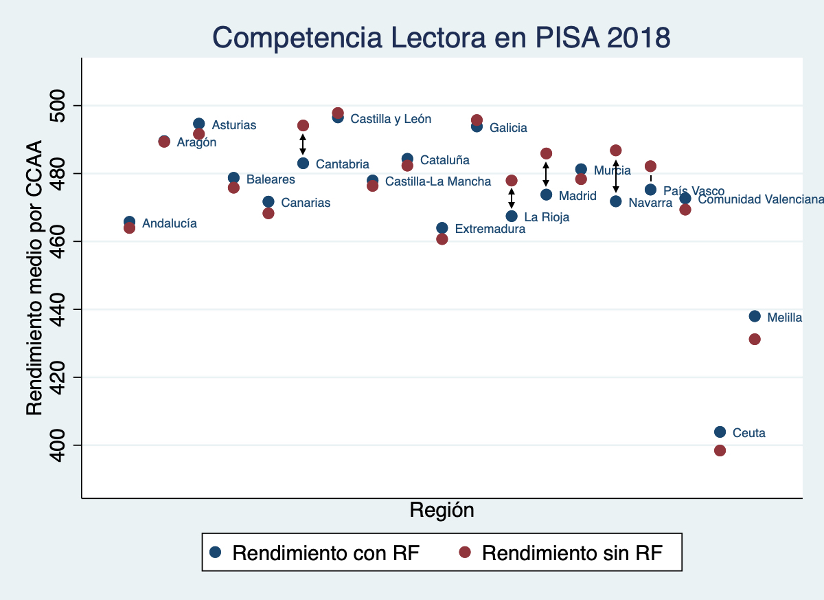
As noted earlier, students’ RF was assessed in a preliminary stage. However, the results of this stage did not determine which items were included in each student’s testlet. Regarding its role in performance measurement, the OECD decided not to incorporate RF results into the different subscales of reading (locating information, understanding, evaluating, and reflecting), but instead to include them in the overall competency score. To date, we have not found any OECD publication explaining precisely how RF was incorporated. Nevertheless, the OECD provides, upon request, alternative plausible values for each student that exclude RF results.

Using these alternative data, we calculated the average performance by region and compared it with the published results that included RF. As shown in Figure 1, the effect of RF is particularly significant in the Autonomous Communities of Cantabria, Madrid, Navarre, La Rioja, and the Basque Country, where the impact diverges from the pattern observed in other regions, whose results are more consistent with each other.

Figure 1

Average reading scores in PISA 2018 by region, depending on whether the effect of reading fluency (RF) is included in the final score.

Note: The numerical values are in Table AI of the Annex.

The PISA 2018 database provides extensive information for each item measuring RF. Most students had to answer 22 items, and for each we have data on their response, the time taken to answer, and whether the response was correct. On average, Spanish students answered 19.33 items correctly, with a median of 20, which was expected given the simplicity of the task.

However, an extraordinary finding emerged when analysing response times, that is, the total time each student spent answering the 22 questions. A significant proportion of students (up to 15% in some Autonomous Communities) completed all 22 items in under 22 seconds, which is far too little time. This was possible because the items were displayed consecutively on the device, and the answers (“yes” or “no”) always appeared in the same position on the screen. As a result, students could simply tap repeatedly on the same box to finish this section in under 22 seconds, typically getting about half of the answers correct. Figure 2 highlights these anomalous response-time patterns in the Autonomous Communities of Madrid, Cantabria, Navarre, La Rioja, and the Basque Country.

Figure 2

Distribution of time spent answering the 22 RF questions in different regions.

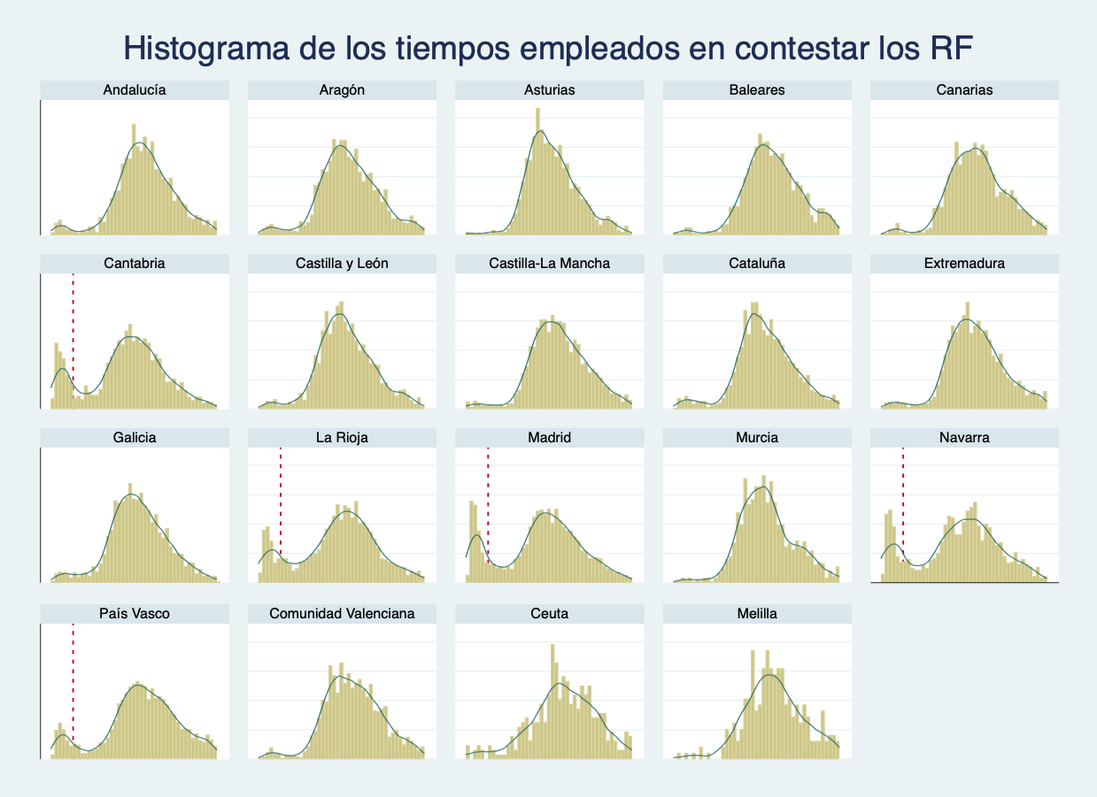
Note: The dashed red line reads 22 seconds

Source: Own elaboration based on PISA2018 data

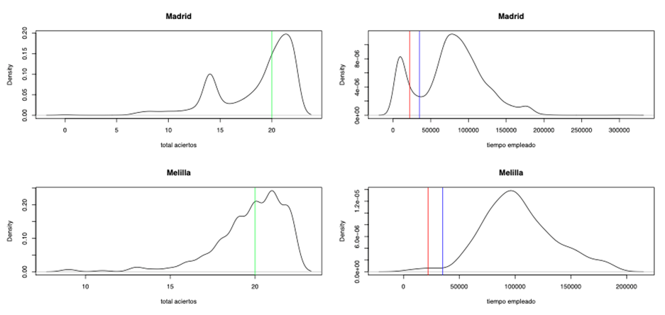
This response-time pattern provided a clue as to what might have happened. We confirmed that the distribution of correct answers on the RF items was also affected by the same anomaly, as shown in Figure 3, which illustrates the distributions for Madrid and Melilla. It was therefore evident that a group of students (significant in some Autonomous Communities) had answered the RF questions “carelessly.” The next step was to identify the characteristics of these students and, most importantly, to assess whether their behaviour had any impact on the overall reading results of the test.

Figure 3

Distribution of the number of correct answers (left) and response times (right) to the RF questions for Madrid and Melilla in PISA 2018.

Note: The red line reads 22 seconds; the blue line reads 35 seconds. The time is measures by milliseconds.

Source: Own elaboration based on PISA2018 data

Methodology

Our first task was to define what we considered anomalous behaviour. To do so, we analysed the response times for the RF items in relation to students’ overall test performance. We then examined how these students were distributed across Autonomous Communities and what their main characteristics were. Finally, using a logit model, we investigated what factors might have triggered such anomalous behaviour.

Dependent Variable: Anomalous Behaviour

We defined anomalous behaviour as a situation where a student performs poorly on the RF stage but achieves strong results in the rest of the test. This required specifying what we mean by “performing poorly” in the preliminary stage and “performing well” in the main test. For the first part, we calculated the variable RF score.

In this study, we classified a student as having performed poorly in the preliminary stage if they obtained a score of fewer than 8 correct answers out of 10 in RF. Table 1 shows the regional distribution (weighted and unweighted) of students who scored below 8 in RF. Approximately 28% of these students were enrolled in schools in the Community of Madrid, 18% in Andalusia, and 11% in Catalonia. The Basque Country and the Valencian Community each accounted for around 6–7%, while the percentages for the remaining regions were below 5%.

Table 1

Distribution by region of students with a score below 8 in RF.

A score below 8 on the RF items could also reflect reading difficulties. Therefore, the criterion for identifying anomalous behaviour combines performance on the RF items with behaviour in the next phase of the test, the core stage. Specifically, we distinguish between students who performed poorly on RF and were then consistently classified at low or medium levels in the core, and those with inconsistent behaviour: students who started poorly on RF but then recovered and achieved a high level in the next stage. The latter represent 16.66% (s.e.: 0.845) of students who scored below 8 on RF and are classified as anomalous—good students who performed unexpectedly poorly on the simple RF items.

Table 2 presents, by Autonomous Community, the percentage of students who, despite scoring below 8 on RF, went on to achieve a high level of performance in the core section. The regions with the highest proportions of such students—between 20% and 30%—are Galicia, the Basque Country, Castile and León, La Rioja, Navarre, Madrid, and Cantabria.

Table 2

Percentage of students exhibiting “abnormal behaviour” in each region

Source: Own elaboration

Independent Variables

To better characterize students with anomalous behaviour, we selected several independent variables at both the student and school levels. These variables are grouped according to their type: categorical variables are presented in Table 3, and continuous variables in Table 4. The study population includes all students who scored below 8 on RF, regardless of their subsequent performance. For categorical variables, we report the percentage of students in each category; for continuous variables, we provide the mean, standard deviation, and their respective standard errors. It should be noted that continuous variables were standardized to have a mean of zero and a standard deviation of one for the full sample of students assessed in PISA 2018.

Table 3

Analysis of Categorical Variables

Note: Estimated percentage of students in each category, together with the standard error of the estimate among students who scored below 8 out of 10 on the RF.

Source: Own elaboration

As shown in Table 3, among students scoring below 8 on RF, 71.84% were enrolled in public schools. Of these, 14.3% reached a high-performance level in the core section, compared with 23.0% among students in private schools. Additionally, 41.4% of students with an RF score below 8 attended schools that brought forward the extraordinary assessment to June. Of these, 23.6% achieved a high level in the core, compared with roughly half that proportion in schools that did not advance the assessment.

Gender differences also emerged: 39.51% of the students scoring below 8 on RF were girls, of whom 21.8% reached a high level in the core. By contrast, only 13.3% of boys achieved this level. Regarding immigration background, 16.5% of students with low RF scores were first- or second-generation immigrants, and of these, 9.2% reached a high level in the core—more than twice the percentage of native students (19%) (Table 3).

Year repetition was another key factor: 41.6% of students with RF scores below 8 had repeated at least one school year, and of these, only 3.8% achieved high performance in the core, compared with 26.1% among students who had not repeated (Table 3). In summary, more than 7 out of 10 students with RF scores below 8 attended public schools, around 60% were boys, and the vast majority were native students (83.5%). Notably, 6 out of 10 of these students were enrolled in schools located in Autonomous Communities that brought forward the extraordinary exams, usually held in September, to June of the 2017–18 academic year.

Table 4 shows the basic statistics for students with an RF score below 8 for the continuous variables included in the model. Two of these variables are school-related: Week, which refers to the week in which the test was taken at the school, and COLT, which measures teacher involvement in the reading assessment. All variables are standardized, with a mean of zero and a standard deviation of one for the group of students participating in PISA 2018.

Table 4

Analysis of continuous variables

Note: Mean and estimated standard deviation of estimates among students who scored below 8 out of 10 on the RF.

Source: Own elaboration

The Week variable takes a high positive mean value, indicating that a large proportion of students in this analysis completed the PISA tests from the middle of the administration period onwards, coinciding largely with the final exams of their academic year. This overlap was particularly pronounced in communities that brought forward their extraordinary assessment tests to June. Regarding teacher involvement in the reading test (COLT), its negative value (-0.1380) reflects a low level of collaboration between teachers and the PISA 2018 assessment.

In the target group of students, variables such as test effort (EFFORT), teacher support in language classes (TEACHSUP), perception of reading difficulty (SCREADDIFF), use of ICT in lessons (ICTCLASS), and school-provided information about the labour market (INFOJOB1) are very close to zero. This suggests that, for these students, these aspects neither improved nor worsened performance compared to the overall average.

For students who answered fewer than 8 items correctly in the Reading Fluency (RF) section, scored significantly above the average in areas such as sense of life purpose (EUDMO), discriminatory school climate (DISCRIM), and use of ICT for schoolwork outside the classroom (HOMESCH) or for social interaction (SOIAICT). Conversely, they performed significantly below the average in global self-efficacy (GCSELFEFF) and experience of being bullied (BEINGBULLIED). Even more negative were their results in reading competence perception (SCREADCOMP), perception of classroom disciplinary climate (DISCLIMA), and socioeconomic status (ESCS). (Table 4).

Log-linear models

We conclude the methodological section by presenting the model we have used to characterize students with “anomalous” behaviour in the test. In fact, given the hierarchical structure of the data and the nature of the dependent variable, the most appropriate approach is a multilevel log-linear model. As in other PISA cycles, the selection of students followed a classic two-stage cluster sampling procedure (school-student). Specifically, we applied the two-stage stratified sequential cluster model (OECD, 2017). First, strata were defined to best represent the target population of each study (in Spain, by Autonomous Community and school ownership). Within each stratum, schools were then selected sequentially and in proportion to their size, measured by the number of eligible students enrolled. Thus, larger schools had a higher probability of selection than smaller ones. In the second sampling stage, 42 students who turned 16 during the test year were selected, regardless of the class or grade in which they were enrolled. If a selected school had 42 or fewer target students, all of them took the test.

As we have already mentioned, the multilevel logistic regression model is the most suitable for this study (Cohen, Cohen, West, & Aiken, 2013; Gelman & Hill, 2006; Merino Noé, 2017; Snijders & Bosker, 2012). This method effectively accounts for variability in large-scale international educational assessments (De la Cruz, 2008; Iñiguez-Berrozpe & Marcaletti, 2018) while avoiding the use of replicated weights present in the databases (Fishbein, Foy, & Yin, 2021).

Therefore, to analyse the effect of predictor variables on the likelihood of anomalous behaviour, we employed multilevel logistic models with fixed effects that reflect the nested structure of the sample. Model estimation was carried out using HLM6© software, applying the Laplace approximation for Bernoulli models (Raudenbush & Bryk, 2002), which enables analyses with binary dependent variables across hierarchical levels.

The equations of the model used are:

Level 1 of the model:

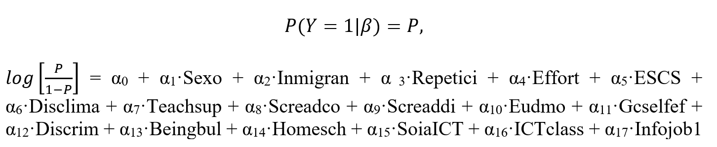
Nivel 2 of the model:

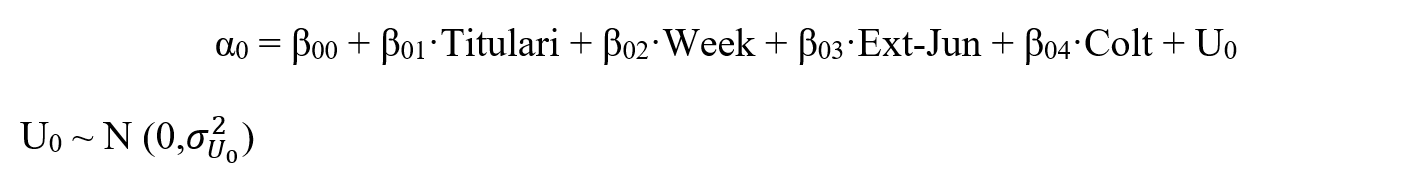
Where,

Y represents whether students exhibit anomalous behaviour or not.

α_i are the fixed coefficients for each predictor variable at level 1.

β_0i are the fixed coefficients for each predictor variable at level 2.

β₀₀ is the regression intercept.

The variables are already presented in Tables 3 and 4.

Results

Table 5 presents the results of the hierarchical log-linear model, in which the dependent variable was the condition “anomalous behaviour.” The model is constructed on two levels: school level and student level. Statistically significant variables were observed at both levels. At the school level, it is worth noting that neither school ownership (TITULARI) nor collaborative support from Spanish teachers (COLT_MEA) had a significant effect on the likelihood of students being classified as exhibiting anomalous behaviour. This suggests that such behaviour is not attributable to specific characteristics of the schools themselves. However, the timing of the PISA test proved relevant: the week in which the school administered the test (WEEK) was statistically significant, with an increase of 10 percentage points in anomalous behaviour among students tested in later weeks. Even more significant was whether the Autonomous Community moved the extraordinary exams forward to June (EXT_JUN), which increased the probability of anomalous behaviour by 87 percentage points. These variables are closely linked: the later the PISA test was taken, the more likely it was to coincide with the end of the school year and, consequently, with students’ final secondary school assessments. Although these factors are exogenous to students, they nonetheless generated reluctance or lack of motivation toward the PISA test, as students were required to take an external assessment while already immersed in the crucial final evaluation of their studies.

At the student level, the adjusted multilevel model examined how and to what extent these school variables influenced individual behaviour. Neither gender (GENDER)—which affected boys and girls in statistically similar proportions—nor students’ perception of teacher support (TEACHSUP), consistent with the school-level variable associated with language teachers, showed statistical significance. By contrast, several other variables did. Notably, repetition of a school year (REPETICI), immigrant status (INMIGRAN), and the discriminatory climate of the school (DISCRIM) all displayed strong effects. Students who had repeated a year were 80 percentage points less likely to exhibit anomalous behaviour, immigrant students 30 percentage points less likely, and students in highly discriminatory school environments 25 percentage points less likely.

Interestingly, students more likely to graduate from 4th year of ESO were more prone to anomalous behaviour, probably due to their lack of interest in the PISA test, which interfered with their main academic focus. Similarly, students with a high self-concept in reading competence (SCREADCO) were 38 percentage points more likely to be classified as anomalous. A considerable number of other variables also showed significant effects within a range of 15–20 percentage points, among them student effort (EFFORT: +19 points), the Socioeconomic and Cultural Index (ESCS: +18 points), a positive school climate (DISCLIMA: +17 points), and self-efficacy in responding to global aspects (GCSELFEF: +20 points). Although these are generally positive contextual indicators, in this case they appear to identify students who did not approach the test with appropriate seriousness or motivation.

Conversely, certain variables reduced the likelihood of anomalous classification. These include perception of difficulty in reading competence (SCREADDI: –13 points) and use of ICT outside school (SOIAICT: –9 %). Both are consistent with the patterns observed in the variables associated with increased probability of anomalous behaviour. These two indicators tend to be linked with lower overall performance, suggesting greater demotivation toward reading skills in general—an effect that was amplified by the particular circumstances of the 2018 PISA administration, as discussed throughout this article.

Table 5

Results of the multilevel analysis

Conclusions

The exclusion of Spain’s results from the PISA 2018 reading assessment in December 2019 was a carefully considered decision by the OECD, following the observation of unexpectedly low performance in certain Autonomous Communities. Although not all of the decline in reading performance can be attributed to the nature and structure of the test, this study has shown that these factors did play a significant role in some cases.

A key element was the presence of an initial section, the Reading Fluency (RF) module, which some students appeared to treat “as if it did not count toward the final score.” This negatively affected the average performance of certain autonomous communities, since the adaptive multistage design of the test, combined with the use of Item Response Theory to calculate individual performance, prevented high-performing students from compensating for a poor start.

The proportion of students who responded “lightly” to RF items—evidenced by abnormally short response times—did not exceed 5% in most regions. However, the percentages were slightly higher in the Basque Country and the Valencian Community (around 7%) and markedly higher in three regions: Catalonia (11.09%), Andalusia (17.7%), and the Community of Madrid (28.32%).

We define students who performed poorly on the RF section but excelled in the subsequent CORE stage as exhibiting anomalous behaviour. In seven regions, the share of such students was close to or above 20%: Cantabria, Castile and León, La Rioja, Community of Madrid, Chartered Community of Navarre, Basque Country, and Galicia (Table 2). A multilevel logistic model allowed us to rule out school ownership, student gender, and language teacher support as relevant factors in anomalous behaviour. By contrast, test administration variables—such as taking the test in the final weeks of the school year (second application window) or advancing extraordinary exams to June—had a clear influence on students’ tendency not to take the RF section seriously. At the individual level, higher reported effort and stronger self-perceptions of reading competence also increased the likelihood of anomalous behaviour.

In other words, high-achieving students who engaged in anomalous behaviour during the PISA 2018 reading test often responded randomly to the RF section—as indicated by their response times—for a variety of possible reasons: they may have been told the section did not count, they may have assumed the items were calibration exercises for the tablet, or they may have dismissed the section as “too easy” to be relevant. Due to the test’s design, however, they were then unable to recover their expected performance levels.

The OECD has already announced its intention to review both the administration of PISA and the impact of the RF modules on student performance. Nevertheless, definitive conclusions will not be possible until reading once again becomes the primary domain assessed. In the meantime, it would be valuable to investigate whether similar patterns of anomalous behaviour occurred in other countries, and to identify the characteristics of the students involved. It would be unrealistic to assume that this phenomenon was unique to Spain.

Given the importance of large-scale international assessments such as PISA—both in shaping public opinion and in guiding potential improvements to educational programs—we consider it essential to highlight the main factors associated with the anomalous behaviour observed among a significant share of students. Accordingly, we recommend:

• Modifying the structure of the test so that it includes RF items but minimizes the possibility of automatic responses. For instance, varying the position of answer choices across items.
• Scheduling the test earlier in the school year, sufficiently far from final exams, to ensure students are not distracted by end-of-year concerns.
• Conducting awareness campaigns to emphasize the importance of the test, underscoring its relevance both nationally (regional comparisons) and internationally (comparisons across countries).

Annex

To assess the impact that this behaviour had on the student´s final average performance, we used data provided by the OECD itself, upon request, on reading performance without taking into account the RF component. In other words, after requesting it from the OECD, we have an alternative score, specifically ten plausible alternative values, to measure the average effect of the RF.

Table AI shows the average value for each region including the RF component (i.e., the values already published by the OECD in its report of July 23, 2020), the average value of performance without considering the RF component, and the difference between the two results.

TABLE AI. Average returns by region, with and without RF, and sample sizes. Differences in average returns presented in Graph I.

Key Terms:

• pv_read_mean: the average reading performance scores for the Autonomous Community published by the OECD
• pv_read_mean: refers to the mean reading performance score of the Autonomous Community excluding the RF results. These data are available on request from the OECD.
• pv_read_N: sample size considered.
• difere: represents the difference between the mean values depending on whether the RF are included or not, calculated as pv_readalt_mean – pv_read_mean.

References

Anghel, E., Khorramdel, L. and von Davier, M. (2024). The use of process data in large-scale assessments: a literature review. Large-scale Assess Educ 12, 13. https://doi.org/10.1186/s40536-024-00202-1

Avvisati, F. et al. (2024), “Item characteristics and test-taker disengagement in PISA”, OECD Education Working Papers, No. 312, OECD Publishing, Paris, https://doi.org/10.1787/7abea67b-en

Bezirhan, U., von Davier, M., and Grabovsky, I. (2020). Modeling Item Revisit Behavior: The Hierarchical Speed–Accuracy–Revisits Model. Educational and Psychological Measurement, 81(2), 363-387. https://doi.org/10.1177/0013164420950556

Cohen, J., Cohen, P., West, S. G., & Aiken, L. S. (2013). Applied multiple regression/correlation analysis for the behavioral sciences. New York: Routledge.

De la Cruz, F. (2008). Modelos multinivel. Epidemiol, 12(3), 1-8. Obtenido de http://sisbib.unmsm.edu.pe/bvrevistas/epidemiologia/v12_n3/pdf/a02v12n3.pdf

Fishbein, B., Foy, P., & Yin, L. (2021). TIMSS 2019 User Guide for the International Database. Boston College, TIMSS & PIRLS International Study Center. Retrieved from timssandpirls.bc.edu/timss2019/international-database/

Gelman, A., & Hill, J. (2006). Data analysis using regression and multilevel/hierarchical models. Cambridge: Cambridge University Press.

Goldhammer F, Scherer R and Greiff S (2020) Editorial: Advancements in Technology-Based Assessment: Emerging Item Formats, Test Designs, and Data Sources. Front. Psychol. 10:3047. doi: 10.3389/fpsyg.2019.03047

Iñiguez-Berrozpe, T., & Marcaletti, F. (2018). Modelos lineales multinivel en SPSS y su aplicación en investigación educativa [Linear multilevel models in SPSS and its application in educational research]. REIRE Revista d’Innovació i Recerca en Educació, 11(1), 26-40. doi:10.1344/reire2018.11.118984

Merino Noé, J. (2017). La potencialidad de la Regresión Logística Multinivel. Una propuesta de aplicación en el análisis del estado de salud percibido. Revista de Metodología de Ciencias Sociales, 36, 177-211. doi:empiria.36.2017.17865

OCDE. (2017). PISA 2015 Technical Report. Retrieved from www.oecd.org/pisa/data/2015-technical-report/

Raudenbush, S. W., & Bryk, A. S. (2002). Hierarchical Linear Models: Applications and data analysis methods. Thousand Oaks: Sage Publications, Inc.

Snijders, T. A., & Bosker, R. J. (2012). Multilevel analysis: An introduction to basic and advanced multilevel modeling. London: Sage.

Weeks, J., von Davier M. and Yamamoto K. (2016): Using response time data to inform the coding of omitted responses. Psychological Test and Assessment Modeling, Volume 58, (4), 671-701

Wise, S.L. (2017), Rapid-Guessing Behavior: Its Identification, Interpretation, and Implications. Educational Measurement: Issues and Practice, 36: 52-61. https://doi.org/10.1111/emip.12165