Reply to “Criticism of the analysis of Construct Validity of the Gifted Rating Scales (GRS 2) Parent Form in Spain; a reply to Tourón et al. (2023)”
Réplica a la “Crítica del análisis de la validez de constructo de la Escala de Detección de alumnos con Altas Capacidades para Padres (GRS 2); réplica a Tourón et al. (2023)”
https://doi.org/10.4438/1988-592X-RE-2024-406-638
Marta Tourón
https://orcid.og/0000-0001-5430-4198
Universidad Internacional de La Rioja - UNIR
Enrique Navarro-Asencio
https://orcid.og/0000-0002-3052-146X
Universidad Complutense de Madrid
Javier Tourón
https://orcid.og/0000-0001-8217-1556
Universidad Internacional de La Rioja - UNIR
Abstract
The objective of this work is to respond to the critical review carried out by Martínez, J. A. (2024) of the study on the construct validity of the Gifted Rating Scales (GRS 2) parent form in Spain, Tourón et al. (2023). The critique mainly focuses on the proposed factorial model, which uses a reflective approach of Confirmatory Factor Analysis (CFA) for measuring the perception of high abilities, while the author in the review proposes a formative approach. This response provides a conceptual clarification of the term giftedness and also replicates the observations made on the validation methodology, focusing on the differences between reflective and formative models and the characteristics of the CFA used. Additionally, evidence is provided to justify the definition of a reflective measurement model through the estimation of a bifactorial model. This model seeks to explain the responses to the items by considering both a general factor and a set of specific factors simultaneously. The results show the importance of a general factor, but without consistent evidence of strict unidimensionality. The presence of a multidimensional structure with four specific factors (cognitive ability, creative ability, social skills, and emotional control) significantly contributes to the explanation of the common variance of the model.
Keywords: gifted rating scales, high ability, construct validity, confirmatory factor analysis, reflective and formative models, bifactor model.
Resumen
El objetivo de este trabajo es responder a la revisión crítica realizada por Martínez, J. A. (2024) del estudio de la validez de constructo de la Escala GRS 2 para padres en España, Tourón et al. (2023). La crítica se centra principalmente en el modelo factorial propuesto, que utiliza una aproximación reflectiva del Análisis Factorial Confirmatorio (AFC) para la medida de la percepción de las altas capacidades. Mientras que en la revisión el autor propone una aproximación formativa. En esta respuesta se lleva a cabo una aclaración conceptual del término giftedness y también se realiza una réplica de las observaciones realizadas a la metodología de validación, poniendo la atención en las diferencias entre modelos reflectivos y formativos y las características del AFC utilizado. Además, se aportan evidencias que justifican la definición de un modelo de medida reflectivo a través de la estimación de un modelo bifactorial. Este modelo trata de explicar las respuestas a los ítems a partir de la consideración, al mismo tiempo, de un factor general y un conjunto de factores específicos. Los resultados muestran la importancia de un factor general, pero sin evidencias consistentes de una unidimensionalidad estricta. La presencia de una estructura multidimensional con cuatro factores específicos (capacidad cognitiva, capacidad creativa, habilidades sociales y control emocional) aporta una parte importante a la explicación de la varianza común del modelo.
Palabras clave: escala de detección, altas capacidades, validez de constructo, análisis factorial confirmatorio, modelos reflectivos y formativos, modelo bifactorial.
Introduction
We appreciate the meticulous study and analysis by Martínez, J. A. of our construct validation work on the Gifted Rating Scales 2 (GRS 2) Parent Form in Spain, in which “several of the methodological procedures and result analysis described by Tourón et al. (2023) are questioned. Both the proposed factorial model based on a reflective view of high-ability measurement and the fit indices used to validate the approximate dimensional structure seriously limit the interpretation of the results.”
We will respond to the observations of Martínez, J. A. following the sequence of their own critique and providing our arguments regarding the work done.
This text aims to address the critique on different aspects related to the model and methodology used in Tourón et al. (2023) to validate the dimensional structure of the GRS 2 in its version for families. Let’s recall that this instrument is a scale for detecting gifted behaviors based on a multidimensional model of high abilities, specifically three dimensions: cognitive abilities, creative and artistic abilities, and socio-emotional skills (Pfeiffer and Jarosewich, 2003). The items included a total of 20, reflect behaviors or characteristics indicative of high ability that can be observed by a parent outside an educational setting. Validation cannot be understood without considering the use of the scores produced by the test. In this case, the GRS 2 parent scale provides information that complements that was provided by teachers to identify these behaviors. Before starting the actual response, it is worth providing some context.
On the Construct and Terminology
There is a preliminary terminological issue that needs to be clarified. The term “giftedness” in English – the language in which the most relevant literature on the subject has been written – means endowed, so the “gifted” is the endowed. The use given to these terms in Spanish has often been “superdotación” and “superdotado” (super-gifted). These terms are not entirely correct and do not correspond with the literature on the subject. Therefore, Tourón (2023) has repeatedly proposed to focus on the substantive dimension of the term and use the words “alta capacidad” (high ability). Thus, ability is the substantive dimension of giftedness. Many current authors (see, e.g., the approaches of Renzulli, Gagné, or Subotnik et al. in Pfeiffer et al., 2018) understand giftedness as a social construct, a designation referring to a multidimensional construct that has various behavioral manifestations in cognitive, affective, social, etc., domains.
Tourón (2020) pointed out that “the conceptual problem in this field of study is enormous and has undesirable consequences for identification and intervention, which is not exclusive to our country. To some extent, it occurs in the Anglo-Saxon realm within the non-researching educational community. A first problem arises from equating terms like ‘gifted’ to ‘superdotado’ (super-gifted, which does not exist in English) and linking it to obtaining an IQ value, generally 130, on one of the standard tests. The main problem here is that the label is equated to a ‘state of being’ or a golden chromosome (Cf. Renzulli and Reis, 2018), so some people possess it, and others do not. This turns the fact of being gifted into a dichotomous variable whose categories are arbitrarily established from a cutoff point [...]. ‘The term “gifted” means that one is exceptional at something, and we prefer to use the word “gifted” as an adjective (e.g., he or she is a gifted pianist, writer, etc.) rather than as a noun (she is gifted). We also prefer to talk about gifted behaviors (adjective) rather than using “the gifted” to represent a state of being (p.185)” [...].
“All current models [...] emphasize the importance of development throughout the person’s life, establishing the relevance of the environment’s impact on such development. [...]. Therefore, it seems sensible to understand that this conceptualization should foreground the need to identify people’s diverse potentials to help them turn them into talents or developed competencies in performance (Cf. Tourón, 2012). Moreover, as Pfeiffer (2017) points out, the term gifted is a social construct, a designation we use to refer to a heterogeneous group of people characterized by having high ability, high performance, or potential to perform,” (p.17-18).
It is necessary to clarify that the GRS 2 scales (in our case, the parent form, although there are two other teacher forms) come from a prior conception of giftedness as a multidimensional reality with external manifestations in behavior. This set of typical observable characteristics of gifted individuals translates into items that parents (in this case) must rate. Thus, it should be expected that items designed to measure a specific dimension are more closely related to each other than if they were developed to measure different dimensions. In this way, the construct dimensions are considered latent variables or dimensions causing the responses to the items, which are considered effects.
Thus, the scale is the measurable operational dimension, albeit imperfectly, that allows estimating the unmeasurable latent traits. This is a clearly reflective approach. The conception of what is measured precedes and is the basis for the measurement instrument.
Finally, it should be noted that this scale, like many others in its genre, does not aim to measure high abilities as a capacity test does, for example, but rather to gather information from other sources (parents) who assess the extent to which certain behaviors or characteristics are present – and to what degree – in the rated individual.
The structure of the scale and its construction follow the conceptualization of the construct it aims to assess but is not an instrument intended to define what giftedness is (see, e.g., Pfeiffer and Jarosewich, 2003; Tourón et al., 2024).
In the work of Tourón et al. (2023), the authors focus on providing psychometric evidence of the construct validity of the Spanish translation of the scale, but they have not participated in the theoretical and operational definition of the construct. It should also be considered that the response to the items included in the scale is the product of the families’ perception of certain behaviors of their children. And that the response to each of these items has an ordinal format using a 6-point Likert scale to identify the frequency of each of these behaviors.
On Validation
The purpose of instrument validation is to collect evidence supporting the interpretation and use of test scores, as stated in the AERA, APA, and NCME manual (2018). Validity refers, as is known, to the degree to which evidence and theory support the interpretations of test scores associated with intended uses (p. 11). Validity evidence can be obtained from five sources: test content, response process, internal structure, relations with other variables, and consequences of test application. In the work of Tourón et al. (2023), evidence of the validity of the internal structure of the items forming the scale and their organization into dimensions is provided, but their purpose is not to estimate factor scores or standardize the instrument.
The methodological critique focuses primarily on defining the measurement model used to collect evidence of the relationship between the items and the latent constructs. In the confirmatory model used in our work, the responses to the scale items are considered dependent variables, i.e., effects produced by the latent factors, which in our model are the exogenous variables, the causes. However, in the review, the role of items and factors is proposed to be reversed, considering formative and not reflective constructs.
In the critical review, the author argues that the most appropriate approach to defining how to calculate factor scores is a formative model where the scores on the different items determine the factor, as opposed to the reflective approach used in the work, as shown in the extended model in the following figure (see Figure I):
FIGURE I. Factorial model and extended model
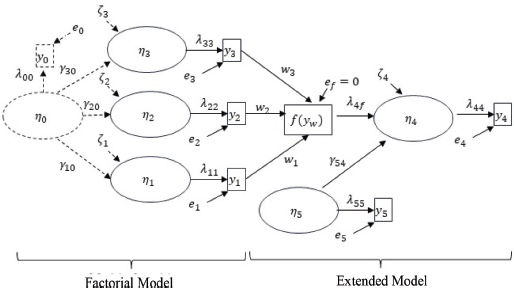
Source: Martínez, J. A. (2024).
The left side of the figure, the factorial model, represents our estimation, and the model on the right is the critique’s proposal against us.
Using one definition or another is a controversial issue in psychometric literature (Murray & Booth, 2018). Opting for one of the models implies making assumptions that range from the theoretical and operational definition of the construct to its empirical validation. Employing a formative approach involves treating the latent factors as endogenous variables, that is, as an effect or result produced by the combination of different indicators, the dependent variable. Therefore, they are not considered independent variables, an exogenous factor that determines how subjects respond to the items.
Murray and Booth (2018) mention five aspects to differentiate between indicators as causes or effects. The first is the direction of causality; in formative models, the items are the cause of the latent factor, and in reflective models, they are the effects, the variables to explain. The second is the changes that the indicators can produce in the construct; in the formative model, any change in the indicator will produce an effect on the value of the construct, whereas, in the reflective model, changes in an indicator should not alter the level of the construct. The third argument refers to whether the construct is the common cause of the set of indicators, which occurs in the case of the reflective model, where the indicators need to be correlated. The fourth is whether the indicators have the same causes and effects, a requirement necessary in reflective models but not in formative ones. Finally, they also mention the interchangeability of the indicators, which, in principle, must be fulfilled in reflective models.
Following Zumbo (2006), the reflective and formative distinction differentiates between measures and indices to treat the indicators or observed variables. In the first case, a change in the latent variable is reflected in changes in the indicators (responses to items are considered dependent or endogenous variables). And in the second, the index is the variable that causes changes in the factor; therefore, they are the causes (independent or exogenous variables). This author points out that conducting a Principal Components Analysis (PCA) is not sufficient evidence to validate a construct from a formative approach, and neither do Confirmatory Factor Analysis (CFA) procedures determine that a reflective construct is present. Still, applying a PCA to a reflective construct is not appropriate. In Bollen and Lennox’s (1991) work, they propose that this differentiation should be explored during content validation, asking experts about the formative or reflective nature of the measure or using think-aloud techniques to collect evidence during a pilot application.
Why a Reflective Model?
The model used in Tourón et al. (2023) seeks to provide psychometric evidence of the dimensional structure of the scale and also the quality of the indicators used for its measurement. In this context, the work studies different models to empirically test different numbers of dimensions and proposes a final model with four dimensions, although a model with two second-order factors is also tested and shows good fit. From this perspective, the existence of unobservable constructs that determine how subjects respond to the items in a test is assumed. It is also assumed that this response is partly explained by the latent construct and partly by measurement error.
It should be noted that the work of Tourón et al. (2023) validates the dimensional structure of the translated GRS 2 instrument, but the authors did not participate in the initial analysis of content validity, which aims to validate the set of indicators and ensure they are a sample of behaviors from the nomological network that defines the construct. This type of validity is usually conducted through expert judgment. However, it is assumed that the GRS 2 scale items meet content validity and that the purpose of the indicators is to represent the behaviors of the measurement construct but may refer to different levels of the same factor.
The description given in the critical review should be supplemented with the following clarifications.
First, Martínez, J. A. mentions that “in line with classical test theory: variation in the latent variable η_1 is manifested in a variation in the observable indicator scaled with parameter λ_11, plus a random error e_1.” (p. 5) as follows:
However, this approach to defining item responses aligns more with the assumptions of Item Response Theory (IRT) than Classical Test Theory (CTT). In CTT, the model focuses on defining the total test score as the sum of the true score and a measurement error:
The dispersion of these errors is an indicator of the precision of observed scores and can be estimated through reliability. Inferences are made using the total test score (scale), calculated from the observed information. In contrast, IRT explicitly defines the behavior of the construct to be measured, the latent trait. Item responses are determined in terms of probability by the level of the construct a subject has.
The CTT model does not include information about the relationship between the latent construct and how to respond to items. Only the concept of true score makes this reference; it is an unobserved part. The difference between the two measurement models can be seen in the following graph (see Figure II):
FIGURE II. Measurement Models in CTT and IRT
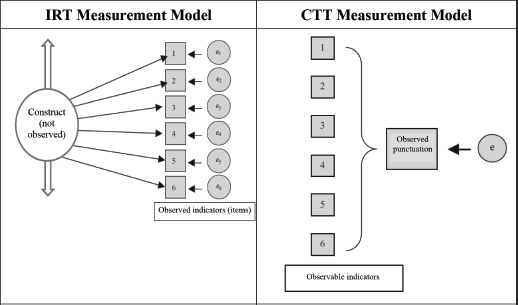
Source: Adapted from Wu, Tam and Jen (2016).
In the IRT model, the arrows indicate the effect of the construct on the probability of responding to the item in a certain way. Therefore, the construct determines the entire response pattern (reflective model). Errors (e) are also represented with circles; they are variables that are not directly observed and indicate the influence on the response of other unknown factors different from the construct we want to measure. The error is a term associated with each item and determines the construct’s ability to explain the response to it.
In CTT, both item responses and the total test score are observed data. The test total is calculated as an aggregation of item responses (sum of correct answers, averages, etc.) (formative model), and the error is associated with this total score, not with each item. The difference between these two models reflects the reflective and formative approach used to define the construct and also the differences between CFA and PCA.
Second, Martínez, J. A. presents a linear approach to factor analysis, while the perspective used in the work of Tourón et al. (2023) due to the ordinal nature of the items and the lack of multivariate normality is nonlinear. Thus, the model to define item responses estimates the score on the construct needed to fall between the different response options. The polychoric correlation matrix was used as an informative element in the factor analysis. Using this type of correlation assumes the existence of an underlying continuous variable (Jöreskog, 1994), and the observed polytomous responses are considered manifestations of respondents exceeding a certain number of cut points or thresholds within that continuum. In this sense, the model estimates these thresholds τ and defines the observed responses in the different ordinal categories through latent continuous variables. Specifically, for an item i with a number of categories c = 0, 1, 2, …, C, the latent variable y* is defined so that:
where τc, τc+1 are the thresholds that determine the cut points in the underlying latent continuous variable, usually spaced at intervals of different widths. Considering this assumption, the correlation of interest for the model is between these continuous variables (polychoric correlation). The analysis procedure is usually carried out in three steps (Jöreskog, 1990; Muthén, 1984). In the first two stages, the thresholds and polychoric correlations are estimated, and in the third stage, these values are fitted to a hypothesized model using some estimation method, mainly DWLS. Model parameters are obtained by minimizing the function that compares the estimated information with the model data.
Third, in the review, Martínez, J. A. mentions a higher-order latent variable as a general factor: “a common conceptualization in this area of knowledge is the first one, as shown, for example, in Pfeiffer et al. (2008), where a multidimensional conception of high abilities with an underlying ‘g’ factor or general ability factor is proposed. It must be acknowledged that Tourón et al. (2023) are very cautious and do not clearly assert this, but they subtly seem to do so when they calculate a ‘total scale mean’ as we will later explain” (p. 6). Here it is worth mentioning that in the validation, a general factor is not tested at any time, but rather a structure with two second-order factors is presented. The first determines the scores on the cognitive and creative factors, and the second for the social and emotional control factors. Additionally, the mean of the set of items calculated in the descriptive statistics section does not aim to show the existence of that general factor; it is just a summary of the data. It should also be remembered that the objective of the work was to provide construct validity evidence but not to estimate scores in the dimensions.
Fourth, related to the above, Martínez, J. A. mentions that “proposing a multidimensional model [...] that reflects an underlying g factor implies from a measurement perspective that the g factor can be measured with the ‘best’ indicator of the ‘best’ dimension, that is, with a single item. This is compatible, as it could not be otherwise, with the reflective view of measurement where the items of a latent variable can be considered interchangeable, indicating that removing one item does not alter the meaning of the latent variable” (p. 7).
In this argument, reference is made to the interchangeability of the indicators used to define the construct and also to the definition of second-order factors. It is unclear whether Martínez, J. A. refers here to the parallelism assumption of CTT scores (Lord and Novick, 1968) or the conceptual parallelism of the indicators defining the construct, which assumes that exchanging one for another does not alter the construct’s meaning (Borsboom et al., 2004). In the first type of parallelism, to estimate the reliability of a test with empirical data, items are considered small parallel parts that reflect the true score and are used for the assessment of internal consistency. Achieving completely parallel measures implies that means, standard deviations, and measurement errors are equivalent, something very complex to achieve in practice. If the same dispersion is not achieved, we are dealing with tau-equivalent measures. Another case of parallelism, essentially tau-equivalent measures, also allows means to vary between different parts by adding a constant. Finally, congeneric measures are the least restrictive and also allow these means to differ by adding or multiplying by a constant. In our validation, a completely parallel structure cannot be assumed because the items of the same construct are a sample of behaviors but may reflect different intensities of that measure. In any case, CFA models allow measures that do not meet strict parallelism, that is, with different factor loadings. Furthermore, the basis of this analysis is the internal consistency of the indicators defining the construct, where correlation is expected. However, the formative approach in PCA does not require the indicators determining the factor to be correlated, and they are assumed not to be interchangeable. CFA allows for indicators with heterogeneous correlation with latent factors. Here, composite reliability (ω) is calculated from the factor loadings to produce more precise estimates than internal consistency procedures like Cronbach’s α.
In second-order factors, it may be more appropriate to define a formative model if the different factors associated with high ability are considered parts of a general factor. Considering the validation results, the two second-order factors (Cognitive-Creative Abilities and Socio-Emotional Skills) defined cannot be considered interchangeable. As the correlation results (0.53) show, they share 25% variability. However, as mentioned earlier, the general factor was not tested in our validation.
Fifth, Martínez, J. A. draws an analogy between intellectual and physical abilities. Here it is worth noting that the GRS scale is a perception instrument; it does not directly measure intellectual ability but infers it from the observation of certain behaviors. Furthermore, indicators for measuring physical abilities are observable and error-free unless the instrument used to collect the measurement does not work correctly. In contrast, perception will be partly determined by the construct but may also be influenced by an unmeasured factor (error).
It may be necessary to measure each indicator once and combine them all to estimate the dimension for measuring physical ability. However, to accurately measure latent dimensions based on item responses, more than one measure of the same behavior is needed. For example, to measure arithmetic ability in primary education math competency, a single exercise may be included to add two amounts or include several with the same purpose in one test. More items will increase the measure’s reliability.
Sixth, Martínez, J. A. also proposes reducing the number of indicators to test this issue; however, as mentioned earlier, the indicators may reflect different levels of the construct, not being considered parallel measures, and will also depend on the conceptual complexity of the measured construct. We insist that indicators can be considered interchangeable in the sense that they are behaviors determined by the same construct, but to measure more accurately, several indicators are needed. Otherwise, the scores would have a lot of measurement errors.
Martínez, J. A. also mentions that “Tourón et al. (2023) seem to consider it positive when they refer to high correlations between each item and the rest, indicating the ‘homogeneity of the data set.’ Moreover, there are examples in the giftedness literature and GRS scales themselves where a halo effect is apparent, obviously affecting validity (e.g., Jabůrek et al., 2020).” (p. 12). However, assuming the possible common cause of responses to the indicators and their internal consistency, this homogeneity is a characteristic of reflective models. The response to the indicators is partly caused by the latent factor, but the model assumes measurement error. That error shows that other factors may determine that response. Martínez, J. A. also mentions that “what is probably happening is that this battery of indicators is measuring different latent variables, i.e., they are not the manifestation of a single latent variable but several.” (p. 12). In this sense, considering the R² values of the items and the averages of variance explained in each factor (AVE), the part explained by latent dimensions is greater than the possible effect of other unconsidered factors. In any case, providing evidence of variables that may determine bias could be another piece of evidence for construct validity.
Finally, seventh, Martínez, J. A. criticizes the methodology, including the use of Exploratory Factor Analysis as a preliminary step to CFA and the fit indices used. Hayduk’s works (2014a and 2014b) are cited as justification for the critique, mentioning that “exploratory factor analysis is incapable of detecting the real structure of the data, i.e., identifying the model that generated those empirical data” (p. 11) and arguing that χ2 can be used even with large sample sizes and that if this test is not passed, the rest of the parameters cannot be interpreted. It is worth mentioning here that the EFA conducted as the first stage does not have a confirmatory purpose; it is used to extract initial information about the number of dimensions and gather evidence of the dimensional structure’s consistency with the confirmatory model. In the validation of the GRS 2 scale, different confirmatory models of three and four dimensions are tested, and decisions are made considering modification indices, for example, changing item 17 from the cognitive to the creative factor.
The statement about the χ2 fit index is too strong, in our opinion. Construct validation procedures in the field of educational measurement and psychometrics point to the need to cautiously interpret this fit index in the context of CFAs. The χ2 statistic tests the null hypothesis that the observed population covariance matrix is equivalent to that produced by the model; however, in Social Sciences, any model is considered an approximation to reality, making that null hypothesis with exact fit unviable (Bentler and Bonett, 1980; Schermelleh-Engel et al., 2003). Hayduk (2014b) indicates that χ2 values are not affected by sample size when the model is correctly specified, but considering the particularity of the models used in Social Sciences, it would not be possible. The same author points out that increasing the sample size increases χ2’s power to detect problems in model specification. The question here is whether, when χ2 is significant, it is really a sufficient indicator to discard the model and commit a Type I error or if that model is the best approximation to reality and the possible bias acceptable. Wang and Wang (2020) argue that the probability of rejecting a model substantially increases when sample sizes increase, even when differences between observed and estimated variance-covariance matrices are small. They note that χ2 values increase when the multivariate normality assumption is not met, and item response distributions are skewed or affected by kurtosis. And also when the number of variables in the model increases. Sufficient reasons not to use it exclusively.
In our case, the estimation uses a weighting of the variance-covariance matrix to estimate χ2 values and standard errors. Remember that since the multivariate normality assumption is not met, WLSMV and the polychoric correlation matrix were used. This estimation method is a version of DWLS (Muthén, 1984) but applying the robust correction of mean and variance to weighted least squares and a scale change (the so-called WLSMV or ULSMV). Although χ2 values are presented in the work, it is not advisable to use it with this type of data (Finney and DiStefano, 2013). The work of Shi et al. (2018) studied how estimation type, sample size, or model complexity affects different χ2 indices and shows a better general performance of robust indices.
Bentler and Bonett (1980) proposed using incremental fit indices such as CFI and TLI to calculate the amount of information gained when comparing models. These indices evaluate the degree to which an estimated model is better than a null model (a model where all observed variables are uncorrelated) in its ability to reproduce the observed variance-covariance matrix. And especially absolute fit measures where it is checked if the defined model corresponds to empirical data. Absolute fit indices such as RMSEA or SRMR do not use a reference null model but make an implicit comparison with a saturated model that exactly reproduces the variance-covariance matrix of observed variables (Hu and Bentler, 1999). The RMSEA index indicates the lack of fit between the specified model in the population and the SRMR estimates the root mean square of residuals.
To conclude this section, it is worth mentioning that any contributions that allow empirically verifying the construct validity of the GRS 2 scale reinforce the instrument’s psychometric quality. To further strengthen the evidence in favor of the model proposed in Tourón et al. (2023), a bifactorial model (Holzinger and Swineford, 1937; Chen et al., 2006) was carried out to check for the existence of a general factor that could be a common cause of the item responses along with the four defined factors.
Bifactorial Model
This proposal defines the shared variance between item responses into two parts: the part explained by a general factor and that determined by a group of specific factors that may be from the same domain. Therefore, it hypothesizes a general factor to explain common variance and, at the same time, multiple factors independently impacting that variance explanation (see Figure III). Since specific factors are interpreted as the variance accounted for beyond the general factor, relationships between general and specific factors are assumed to be orthogonal (uncorrelated).
FIGURE III. Bifactorial Model
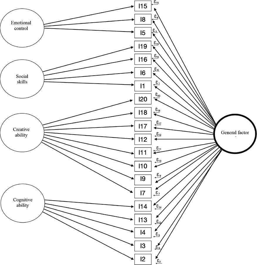
Source: Compiled by the authors.
Chen and Zhang (2018) point out that the ability to study specific factors independently of the general factor is essential for better understanding theoretical assertions. For example, if a proposed specific factor did not explain a substantial amount of variance beyond the general factor, small and insignificant factor loadings in the specific factor, as well as insignificant specific factor variance in the bifactorial model, would be observed. This would indicate that the specific factor does not provide an explanation for the variance beyond the general factor.
To carry out a model evaluation after obtaining the model fit for both unidimensional and bifactorial models, they can be directly compared through the difference between CFI indices (ΔCFI) since the unidimensional model is hierarchically nested within the bifactorial model (Reise, 2012). This index is calculated as follows:
Where CFI_M1 equals the CFI value obtained for model 1, and CFI_M0 equals the CFI value obtained for model 0. This index is more stable under different conditions such as sample size, amount of error, number of factors, and number of items, and values equal to or below .01 are recommended to confirm equivalence (Meade et al., 2008).
For reliability, four versions of the omega coefficient (or composite reliability) can be used: total omega for the general factor (ωt), omega for each subdimension (ωs), and hierarchical omega coefficients that can also be calculated for the general factor (ωht) and each subdimension (ωhs). McDonald’s omega coefficient (1999) is a type of reliability based on factor analysis results, appropriate when dealing with congeneric measures (different factor loadings), estimating the proportion of observed variance attributable to the model’s factors:
The denominator contains all sources of variance in the model, the common variance produced by all factors in the general model and subdimensions, plus specific error variance. The numerator includes only those sources of common variance. It can also be calculated for each subdimension:
In this case, the factor loadings and errors are from the items corresponding to the subdimension. And to determine the proportion of total score variance due solely to the general factor, the hierarchical omega coefficient is used, calculated by dividing the sum of the general factor loadings squared by the total variance, considering common variance and error:
The variance due to subdimensions is considered here part of the measurement error; a coefficient of .80 or higher indicates that scores can be considered essentially unidimensional, considering the general factor as the main source of variance. Furthermore, how much each dimension contributes to common variance can be determined once the general factor is controlled with the following formula (Reise, 2012):
As in the case of total variance, only the factor loadings and errors of the items that make up the subdimension are used. As a reference, the cutoff points mentioned by Smits et al. (2014) can be used, where values equal to or greater than .30 can be considered significant, those below up to .20 moderate, and below .20 low.
From this perspective, the Explained Common Variance (ECV) index is used to contrast the unidimensionality of scales based on the factor loadings of the general factor and subdimensions (Reise et al., 2013) as follows:
Thus, it is the proportion of variance explained by the general factor divided by the variance explained by that factor and the subdimensions. High values indicate the significant importance of the general factor, but setting cutoff points is not straightforward. Values of .70 or higher are suggested to consider unidimensionality (Rodríguez et al., 2016). This indicator can also be calculated at the item level to identify those where the influence of the general factor is very strong. Authors like Stucky and Edelen (2014) propose values above .80 or .85.
To interpret the ECV unidimensionality index, it is recommended to also calculate the Percentage of Uncontaminated Correlations (PUC) (Rodríguez et al., 2016). This index, along with ECV, informs about the potential bias of forcing multidimensional data into a unidimensional model by calculating how many correlations may be moderating the effects of the general factor. PUC can be defined as the number of uncontaminated correlations divided by the number of unique correlations:
IG is the number of items loading on the general factor and Is is the number of items loading on each specific factor. When PUC values are above .80, ECV values are not very relevant as they indicate that the factor loadings of the unidimensional model will approximate those obtained in the general factor of the bifactorial model. However, if PUC values are below .80, ECV values above .60 are needed to consider unidimensionality. And if PUC values are very high (> .90), unbiased unidimensional estimates can be obtained even when the ECV value is low (Reise, 2012).
Other indicators that can help demonstrate the model’s quality is the construct replicability index (H), used to indicate the capacity of the set of items to define each factor. This index allows assessing whether the set of items representing each latent variable is adequate, calculated as follows:
Thus, it is a sum of the rate of variance explained by the latent variable divided by the measurement error, i.e., the proportion of the construct’s variability explained by its indicators. Values of .70 or more indicate that the latent variable is well-defined by its indicators and will have stability in different studies (Rodríguez et al., 2016).
Finally, the factor loadings of the bifactorial model are analyzed and compared with the results of the general factor obtained in the purely unidimensional model (M3, see Table I). Based on the differences between the factor loading values of each item from the two models, the relative parameter bias (SRP) is calculated:
The average of this index informs about the bias that can occur when adjusting a unidimensional model when that assumption is not met. Values above 15% would indicate this possible bias (Rodríguez et al., 2016). Additionally, as Ferrando and Lorenzo-Seva (2018) point out, if in the bifactorial model, the general factor accumulates high loadings and, in the dimensions, the average of their loadings does not exceed .30, it can be another indicator of the unidimensional structure of the measure.
Results
First, the fit values of the bifactorial model are compared with some of those tested in Tourón et al. (2023). Specifically, the results of the original model (M1), the unidimensional model (M3), the proposed model (M6), and its version with two second-order factors (M8) are presented. Finally, the new bifactorial model (M9).
TABLE I. Fit indices of models and difference between the bifactorial model and the one proposed in Tourón et al. (2023)
Indices |
M1 |
M3 |
M6 |
M8 |
M9 |
Difference (Δ) M9-M8 |
AFC |
3 |
1 |
|
|
||
χ2 |
2048 |
6833 |
1596 |
1601 |
1760 |
|
gl |
167 |
170 |
164 |
165 |
150 |
|
p |
<.001 |
<.001 |
<.001 |
<.001 |
<.001 |
|
χ2/gl |
12.263 |
40.194 |
9.732 |
9.703 |
11.733 |
|
SRMR |
0.086 |
0.154 |
0.074 |
0.074 |
0.081 |
0.007 |
RMSEA |
0.101 |
0.189 |
0.089 |
0.089 |
0.098 |
0.009 |
CFI |
0.968 |
0.867 |
0.976 |
0.976 |
0.973 |
-0.003 |
TLI |
0.964 |
0.851 |
0.972 |
0.972 |
0.966 |
-0.006 |
GFI |
0.978 |
0.91 |
0.983 |
0.983 |
0.981 |
-0.002 |
Source: Compiled by the authors.
The bifactorial model, considering the differences in incremental and absolute fit indices with the proposed model (M6), can be considered equivalent in its explanatory capacity. It also shows a better fit than the purely unidimensional model (M3).
Second, the absolute and hierarchical omega values for the general factor and subdimensions are presented in the following Table II:
TABLE II. Omega and Hierarchical Omega of Factors (General and Specific)
|
General F. |
Cognitive |
Creative |
Social |
Emotional |
ω |
0.941 |
0.880 |
0.921 |
0.826 |
0.789 |
ωh |
0.669 |
0.427 |
0.566 |
0.495 |
0.509 |
The omega (ω) values indicate the reliability of each factor, and the hierarchical omega coefficient (ωh) shows the portion attributable to each factor in explaining the total variance. As seen, the ωh value of the general factor, although below 0.70, shows a significant contribution. The factors also contribute to explaining the total variance with ωh values around 50%.
Comparing the ω and ωh results for the general factor, if 66.9% of the variability is determined by that factor, the remaining 27.2% is caused by differences in the specific factors. The rest, 5.9%, is therefore attributed to measurement error.
Third, the unidimensionality index ECV is 0.71, indicating that 71% of the common variance is explained by the general factor and the remaining 29% by the subdimensions. Recall that values of 0.80 indicate unidimensionality, and values close to 0.70 could also be indicative of that possibility. However, the item-level ECV index detects only one item with a value above 0.80, item 17, as shown in the following Table III:
TABLE III. Item-Level Common Variance Explained Index (I_ECV)
Item |
I_ECV |
Item |
I_ECV |
I1 |
0.469 |
I11 |
0.419 |
I2 |
0.455 |
I12 |
0.632 |
I3 |
0.727 |
I13 |
0.471 |
I4 |
0.433 |
I14 |
0.498 |
I5 |
0.172 |
I15 |
0.256 |
I6 |
0.507 |
I16 |
0.469 |
I7 |
0.172 |
I17 |
0.805 |
I8 |
0.780 |
I18 |
0.485 |
I9 |
0.209 |
I19 |
0.193 |
I10 |
0.395 |
I20 |
0.270 |
Source: Compiled by the authors.
Additionally, the Percentage of Uncontaminated Correlations (PUC) is 0.75. A value below 0.80 combined with an ECV of 0.669 raises doubts about the presence of a single general factor.
Fourth, the construct replicability index H is shown in the following Table IV:
TABLE IV. Construct Replicability Index (H)
|
General F. |
Cognitive |
Creative |
Social |
Emotional |
H |
0.869 |
0.697 |
0.865 |
0.678 |
0.721 |
Recall that this index shows the representational capacity that the set of items must have to define each factor. In all cases, values close to or higher than 0.7 are achieved. Therefore, 70% or more of the variability of each latent factor is determined by the indicators that compose it and can be considered acceptable.
Finally, as shown in Table V, the factor loadings show moderate loadings for the general factor, between 0.3 and 0.6, but all are significant. The values in the subdimensions, although similar, are slightly higher and also significant, as shown in the following table. On average, both the general factor and the subdimensions have considerable factor loadings, exceeding the proposed cutoff point of 0.3. In the case of the general factor, it is very close to 0.5, and in the subdimensions, it is slightly above that value and with very similar levels among them.
TABLE V. Standardized Factor Loadings of the Bifactorial Model (M9) and the Unidimensional Model (M3), R², and Relative Parameter Bias Index (SRP)
|
λ* |
λ* |
||||||
Item |
General F. |
Cognitive |
Creative |
Social |
Emotional |
R² |
Unidim. |
SRP |
I2 |
0.602 |
0.659 |
|
|
|
0.797 |
0.696 |
0.034 |
I3 |
0.632 |
0.387 |
|
|
|
0.549 |
0.602 |
0.156 |
I4 |
0.504 |
0.577 |
|
|
|
0.587 |
0.574 |
0.047 |
I13 |
0.595 |
0.631 |
|
|
|
0.751 |
0.692 |
0.139 |
I14 |
0.404 |
0.406 |
|
|
|
0.328 |
0.399 |
0.066 |
I7 |
0.339 |
|
0.745 |
|
|
0.670 |
0.740 |
0.054 |
I9 |
0.407 |
|
0.792 |
|
|
0.793 |
0.829 |
1.183 |
I10 |
0.577 |
|
0.714 |
|
|
0.842 |
0.897 |
0.169 |
I11 |
0.570 |
|
0.671 |
|
|
0.775 |
0.854 |
1.037 |
I12 |
0.438 |
|
0.334 |
|
|
0.303 |
0.508 |
0.555 |
I17 |
0.461 |
|
0.227 |
|
|
0.264 |
0.467 |
0.498 |
I18 |
0.520 |
|
0.536 |
|
|
0.558 |
0.701 |
0.160 |
I20 |
0.432 |
|
0.711 |
|
|
0.692 |
0.773 |
0.163 |
I1 |
0.446 |
|
|
0.475 |
|
0.424 |
0.431 |
0.012 |
I6 |
0.517 |
|
|
0.510 |
|
0.527 |
0.489 |
0.010 |
I16 |
0.548 |
|
|
0.583 |
|
0.639 |
0.527 |
0.038 |
I19 |
0.341 |
|
|
0.698 |
|
0.604 |
0.390 |
0.013 |
I5 |
0.362 |
|
|
|
0.793 |
0.761 |
0.386 |
0.348 |
I8 |
0.544 |
|
|
|
0.289 |
0.379 |
0.452 |
0.144 |
I15 |
0.390 |
|
|
|
0.665 |
0.595 |
0.394 |
0.789 |
Average |
0.481 |
0.532 |
0.591 |
0.567 |
0.582 |
0.592 |
0.590 |
0.281 |
*All parameters are significant (p<.001). Source: Compiled by the authors.
Observing the factor loadings in the table above, for 5 out of the 20 items that make up the scale, the value is higher in the general factor than in the subdimensions. These are items 3, 6, 8, 12, and 17, belonging to different subdimensions of the model. The bifactorial model (M9) explains approximately 60% of the data variability, while M3 explains 38%. Finally, regarding the relative parameter bias (SRP), the average value is close to 30%; therefore, exceeding the 15% limit indicates substantial differences in the effects of that general factor in the two models.
Conclusions
Reflective models cannot be considered superior to formative ones, or vice versa. Both can be alternatives in the study of construct validity (Bollen and Diamantopoulos, 2017). However, in the specific case of the GRS scale, the reflective option used in the construct validity study of Tourón et al. (2023) fits its theoretical and operational definition. Considering the results of the bifactorial model, the presence of a general factor as a cause of much of the variability in the item responses is confirmed, as well as a multidimensional structure of specific factors that contributes another part to the common variance of the model (cognitive ability, creative ability, social skills, and emotional control).
The value of the unidimensionality index (ECV) and the percentage of uncontaminated correlations (PUC), both below 0.80, do not clearly show the presence of a single general factor to explain the item responses. However, these results show the importance of that factor and the influence of the subdimensions in explaining the differences. As indicated by the hierarchical omega coefficients of the subdimensions, all close to or above 0.50, these can be considered significant effects (Smits et al., 2014). Reise et al. (2013) point out that with PUC values below 0.70, an ECV value of the general factor above 0.60, and a hierarchical omega above 0.70 suggest the presence of some multidimensionality, although they do not completely rule out interpreting the scale as unidimensional.
The intensity differences between the factor loadings of each factor demonstrate the congeneric nature of the measures, but the results indicate the presence of a common cause that determines much of the variance in the variance-covariance matrix. This general factor identified in the factorial model determines approximately 70% (ECV = 0.71) of the common variance, so the interchangeability of the indicators considered behaviors caused by the same construct can be maintained. This issue is crucial for defining a reflective measurement model (Murray and Booth, 2018). The rest of the common variance, approximately 30%, is produced by the differences in the results of the subdimensions.
The factor loadings have all been significant, both in the general factor and in the subdimensions. The item-level ECV indices (see Table III) show that the general factor determines part of the item responses, but only for item 17 does that contribution exceed 80%. For items 3 and 8, the general factor explains approximately 75%. For 10 of the items, the contribution ranges from 41% to 60%, and for the remaining seven items, it is approximately 20% to 40%. Therefore, in most items, the influence of the general factor combines with the impact of the subdimensions.
Additionally, the construct replicability indices show good results with values close to or above 0.70. Therefore, the set of indicators that make up each latent variable explains sufficient variability and will have stability in different studies (Rodríguez et al., 2016).
Considering the factor loadings in the bifactorial model show sufficient size in both the general factor and the subdimensions, with average values close to or above 0.50, indicating the importance of the complete model (Ferrando and Lorenzo-Seva, 2018). The relative parameter bias index (SRP) also indicates that the factor loadings of the general factor in the bifactorial model differ from those in the unidimensional model. Therefore, not considering the multidimensional structure introduces bias in the estimates.
We appreciate the thorough critical review conducted and hope to have satisfactorily addressed most of the objections raised. We will consider the new avenues of consideration that arise from this discussion and reanalysis of our data. Finally, we thank the journal editor for accepting to include these works following our original one, as we understand that these debates and methodological differences advance and improve scientific work.
Bibliographic references
American Educational Research Association, American Psychological Association, & National Council on Measurement in Education. (2018). Standards for Educational and Psychological Testing (M. Lieve Trans.). AERA. American Educational Research Association.
Bentler, P. M., & Bonett, D. G. (1980). Significance tests and goodness of fit in the analysis of covariance structures. Psychological Bulletin, 88(3), 588–606. https://doi.org/10.1037/0033-2909.88.3.588
Bollen, K. A., & Diamantopoulos, A. (2017). In defense of causal-formative indicators: A minority report. Psychological Methods, 22(3), 581–596. https://doi.org/10.1037/met0000056
Bollen, K. A., & Lennox, R. (1991). Conventional wisdom on measurement: A structural equation perspective. Psychological Bulletin, 110(2), 305–314. https://doi.org/10.1037/0033-2909.110.2.305
Borsboom, D., Mellenbergh, G. J., & Van Heerden, J. (2004). The Concept of Validity. Psychological Review, 111(4), 1061–1071. https://doi.org/10.1037/0033-295X.111.4.1061
Chen, F. F., West, S. G., & Sousa, K. H. (2006). A Comparison of Bifactor and Second-Order Models of Quality of Life. Multivariate Behavioral Research, 41(2), 189–225. https://doi.org/10.1207/s15327906mbr4102_5
Chen, F. F., & Zhang, Z. (2018). Bifactor Models in Psychometric Test Development. In P. Irwing, T. Booth, & D. J. Hughes (Eds.), The Wiley Handbook of Psychometric Testing: A Multidisciplinary Reference on Survey, Scale, and Test Development (pp. 325-345). https://doi.org/10.1002/9781118489772.ch12
Ferrando, P. J., & Lorenzo-Seva, U. (2018). Assessing the Quality and Appropriateness of Factor Solutions and Factor Score Estimates in Exploratory Item Factor Analysis. Educational and Psychological Measurement, 78(5), 762-780. https://doi.org/10.1177/0013164417719308
Finney, S. J., & DiStefano, C. (2013). Nonnormal and categorical data in structural equation modeling. In G. R. Hancock & R. O. Mueller (Eds.), Structural equation modeling: A second course (2nd ed., pp. 439–492). IAP Information Age Publishing.
Hayduk, L. A. (2014a). Seeing perfectly-fitting factor models that are causally misspecified: Understanding that close-fitting models can be worse. Educational and Psychological Measurement, 74(6), 905-926. https://doi.org/10.1177/0013164414527449
Hayduk, L. A. (2014b). Shame for disrespecting evidence: The personal consequences of insufficient respect for structural equation model testing. BMC: Medical Research Methodology, 14, 124. https://doi.org/10.1186/1471-2288-14-124
Holzinger, K. J., & Swineford, F. (1937). The Bi-factor method. Psychometrika, 2, 41–54. https://doi.org/10.1007/BF02287965
Hu, L., & Bentler, P. M. (1999). Cutoff criteria for fit indexes in covariance structure analysis: Conventional criteria versus new alternatives. Structural Equation Modeling: A Multidisciplinary Journal, 6(1), 1-55. https://doi.org/10.1080/10705519909540118
Jabůrek, M., Ťápal, A., Portešová, Š., & Pfeiffer, S. I. (2020). Validity and Reliability of Gifted Rating Scales-School Form in Sample of Teachers and Parents – A Czech Contribution. Journal of Psychoeducational Assessment, 39(3), 361–371. https://doi.org/10.1177/0734282920970718
Jöreskog, K. G. (1990). New developments in LISREL: Analysis of ordinal variables using polychoric correlations and weighted least squares. Quality and Quantity, 24, 387–404.
Jöreskog, K. G. (1994). On the estimation of polychoric correlations and their asymptotic covariance matrix. Psychometrika, 59, 381–389.
Lord, F. M., & Novick, M. R. (1968). Statistical theories of mental test scores. Addison-Wesley.
McDonald, R. P. (1999). Test Theory: A Unified Treatment (1st ed.). Psychology Press. https://doi.org/10.4324/9781410601087
Meade, A. W., Johnson, E. C., & Braddy, P. W. (2008). Power and sensitivity of alternative fit indices in tests of measurement invariance. Journal of Applied Psychology, 93(3), 568-592. https://doi.org/10.1037/0021-9010.93.3.568
Murray, A. L., & Booth, T. (2018). Causal Indicators in Psychometrics. In P. Irwing, T. Booth, and D. J. Hughes (Eds.), The Wiley Handbook of Psychometric Testing. https://doi.org/10.1002/9781118489772.ch7
Muthén, B. (1984). A general structural model with dichotomous, ordered categorical, and continuous latent variable indicators. Psychometrika, 49(1), 115–132. https://doi.org/10.1007/BF02294210
Pfeiffer, S. (2017). Identificación y evaluación del alumnado con altas capacidades: Una guía práctica. La Rioja: UNIR Editorial.
Pfeiffer, S. I., & Jarosewich, T. (2003). GRS: Gifted Rating Scales. Psychological Corporation.
Pfeiffer, S. I., Petscher, Y., & Kumtepe, A. (2008). The Gifted Rating Scales-School Form: A Validation Study Based on Age, Gender, and Race. Roeper Review, 30(2), 140–146. https://doi.org/10.1080/02783190801955418
Pfeiffer, S. I., Shaunessy-Dedrick, E., & Foley-Nicpon, M. (Eds.). (2018). APA handbook of giftedness and talent. American Psychological Association. https://doi.org/10.1037/0000038-000
Reise, S. P. (2012). The rediscovery of bifactor measurement models. Multivariate Behavioral Research, 47, 667–696. https://doi.org/10.1080/00273171.2012.715555
Reise, S. P., Scheines, R., Widaman, K. F., & Haviland, M. G. (2013). Multidimensionality and Structural Coefficient Bias in Structural Equation Modeling: A Bifactor Perspective. Educational and Psychological Measurement, 73(1), 5-26. https://doi.org/10.1177/0013164412449831
Renzulli, J. S., & Reis, S. M. (2018). The three-ring conception of giftedness: A developmental approach for promoting creative productivity in young people. In S. I. Pfeiffer, E. Shaunessy-Dedrick, & M. Foley-Nicpon (Eds.), APA Handbook of Giftedness and Talent (pp. 185–199). American Psychological Association. https://doi.org/10.1037/0000038-012
Rodríguez, A., Reise, S. P., & Haviland, M. G. (2016). Evaluating bifactor models: Calculating and interpreting statistical indices. Psychological Methods, 21(2), 137–150. https://doi.org/10.1037/met0000045
Schermelleh-Engel, K., Moosbrugger, H., & Müller, H. (2003). Evaluating the fit of structural equation models: Tests of significance and descriptive goodness-of-fit measures. Methods of Psychological Research Online, 8(2), 23-74.
Shi, D., DiStefano, C., McDaniel, H. L., & Jiang, Z. (2018). Examining Chi-Square Test Statistics Under Conditions of Large Model Size and Ordinal Data. Structural Equation Modeling: A Multidisciplinary Journal, 25(6), 924-945. https://doi.org/10.1080/10705511.2018.1449653
Smits, I. A., Timmerman, M. E., Barelds, D. P., & Meijer, R. R. (2014). The Dutch symptom checklist-90-revised. European Journal of Psychological Assessment, 31(4), 263-271. https://doi.org/10.1027/1015-5759/a000233
Stucky, B. D., & Edelen, M. O. (2014). Using hierarchical IRT models to create unidimensional measures from multidimensional data. In S. P. Reise & D. A. Revicki (Eds.), Handbook of Item Response Theory Modeling: Applications to Typical Performance Assessment (pp. 183-206). Routledge/Taylor & Francis.
Tourón, J. (2012). ¿Superdotación o alta capacidad? Retrieved from https://www.javiertouron.es/superdotacion-o-alta-capacidad/
Tourón, J. (2020). Las altas capacidades en el sistema educativo español: reflexiones sobre el concepto y la identificación: Concept and Identification Issues. Revista de Investigación Educativa, 38(1), 15–32. https://doi.org/10.6018/rie.396781
Tourón, J. (2023). ¿Puede una escuela inclusiva ignorar a sus estudiantes con altas capacidades? enTERA2.0, 10, 24-46.
Tourón, M., Navarro-Asensio, E., & Tourón, J. (2023). Validez de Constructo de la Escala de Detección de alumnos con Altas Capacidades para Padres (GRS 2) en España. Revista de Educación, 402, 55-83. https://doi.org/10.4438/1988-592X-RE-2023-402-595
Tourón, M., Tourón, J., & Navarro-Asencio, E. (2024). Validación española de la Escala de Detección de altas capacidades «Gifted Rating Scales 2 (GRS 2-S) School Form» para profesores. Estudios Sobre Educación, 46, 33-55. https://doi.org/10.15581/004.46.002
Wang, J., & Wang, X. (2020). Structural Equation Modeling: Applications Using Mplus (2nd ed.). John Wiley & Sons Ltd.
Wu, M., Tam, H. P., & Jen, T. H. (2016). Educational measurement for applied researchers. Theory into Practice. https://doi.org/10.1007/978-981-10-3302-5
Zumbo, B. D. (2006). 3 validity: foundational issues and statistical methodology. In C. R. Rao & S. Sinharay (Eds.), Handbook of Statistics: Vol. 26. Psychometrics (pp. 45-79). Elsevier Science. https://doi.org/10.1016/S0169-7161(06)26003-6
Contact address: Marta Tourón Porto, Universidad Internacional de La Rioja - UNIR. Avd. de La Paz, 137. 26006 Logroño La Rioja. E-mail: marta.tporto@unir.net